Sometimes when you are looking at fluid flowing through a system you will notice that the cross-sectional area changes. This is an example of confined flow. When you are analyzing this type of problem you can use Bernoulli equation to express the change in the fluids characteristics as it flows from one point to another.
First, let take a look at the general Bernoulli equation along a streamline.
(Eq 1) $p_1 + \frac{1}{2}ρv_1^2 + γz_1 = p_2 + \frac{1}{2}ρv_2^2 + γz_2$
$p$ = thermodynamic pressure
$ρ$ = fluid density
$v$ = fluid velocity
$γ$ = specific weight
$z$ = fluid height
Recall, to use Bernoulli equation you will need to be able to satisfy a few assumptions. These assumptions are the following. First, the fluid must be considered inviscid. Second, the fluid is incompressible. Finally, third, the fluid is in a steady state. If you are an able to satisfy these conditions than you will have inaccuracies in your result.
Continuity Equation
For a problem where you are analyzing confined flow you will also need to use the continuity equation. The reason why is because when there is an increase in velocity there is a decrease in pressure and vice versa. As a result there will be two unknowns for this type of problem. The continuity equation will provide you will the necessary tool to solve for this additional unknown. Refer to the equation below.
(Eq 2) $A_1v_1 = A_2v_2~or~Q_1 = Q_2$
$A$ = cross-sectional area
$Q$ = flowrate
The above equation in the continuity equation for an incompressible fluid. If the fluid is compressible then you will need to add a density term on each side of the equation. Finally, this equation is derived from the conservation of mass.
Confined Flow
As mentioned above a confined flow problem is when the cross-sectional area that the fluid is flowing through changes from one point to another point. This can be see in the image below.
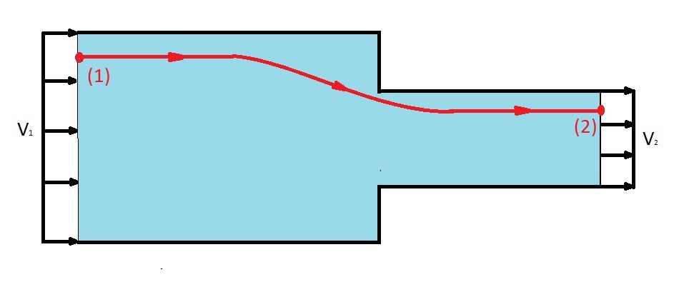
First let’s take a look at point 1. At point 1 there will a thermodynamic pressure as well as dynamic pressure. There is however no hydrostatic pressure due to a fluid height. As a result the left side of Bernoulli equation would look like the following.
$p_1 + \frac{1}{2}ρv_1^2$
Now let’s take a look at point 2. As with point 1 there will be a thermodynamic pressure and a dynamic pressure at this point. In addition there will be no hydrostatic pressure due to fluid height. Hence the right side of Bernoulli equation would be the following.
$p_2 + \frac{1}{2}ρv_2^2$
The resulting Bernoulli equation will become the following.
$p_1 + \frac{1}{2}ρv_1^2=p_2 + \frac{1}{2}ρv_2^2$
Now what if we know what the thermodynamic pressure and fluid velocity is at point 1, but don’t know either one of these values at point 2? This would result in two unknowns, meaning that we will have take advantage of the continuity equation. So first let solve for $v_2$ using the continuity equation.
$v_2 = v_1\frac{A_1}{A_2}$
As a result we are now left with one unknown $p_2$. We can now combine the continuity equation and Bernoulli equation find the thermodynamic pressure $p_2$.
$p_2 = p_1+\frac{1}{2}ρv_1^2\left(1-\left(\frac{A_1}{A_2}\right)^2\right)$