There are many cases where standard fluid mechanics equations can be used to solve a problem. However, there are also many cases where equations alone cannot obtain a solution. Instead a combination of dimensional analysis and experimental data will need to be used.
When you are using experimental data you will need to understand the concepts of similitude. Similitude will allow you to use experimental data from a carefully controlled system in a laboratory and than apply it to another similar system outside of the laboratory. Laboratory systems are known as models. In turn, these models will give you the ability to derive an empirical formula to help predict how an uncontrolled system will behave.
Applying Dimensional Analysis
Let’s take a look at an incompressible Newtonian fluid that has a steady flow as it moves through a long, smooth walled, horizontal, circular pipe. One thing that we would be interested in is the pressure drop per unit length. Even though this is a fairly straight forward problem it cannot be solved without first using experimental data. Hence, an experimental study will need to be planned. In order to do this we will first need to consider what variables will have an effect on the pressure drop. For instance, in this case it is expected that pipe diameter, $D$, fluid density, $ρ$, fluid viscosity, $μ$, and the fluid velocity, $v$, will have an effect on the pressure drop. As a result, the following relationship will be applied.
(Eq 1) $Δp_l=f(D,ρ,μ,v)$
In turn, this expression is simply indicating that these variables will have a mathematical effect on the pressure drop. However, we still do not know the nature of the function. To determine this you will need to use experimental data.
Obtaining Experimental Data
The experimental data must be collected in a controlled manner. In order to do this, only one variable, such as velocity, can be changed at a time while the other variables must remain at a known constant. You will then record the pressure drop. As a result, this will allow us to graphically represent the variable of interest vs pressure drop which can be seen in the images below.
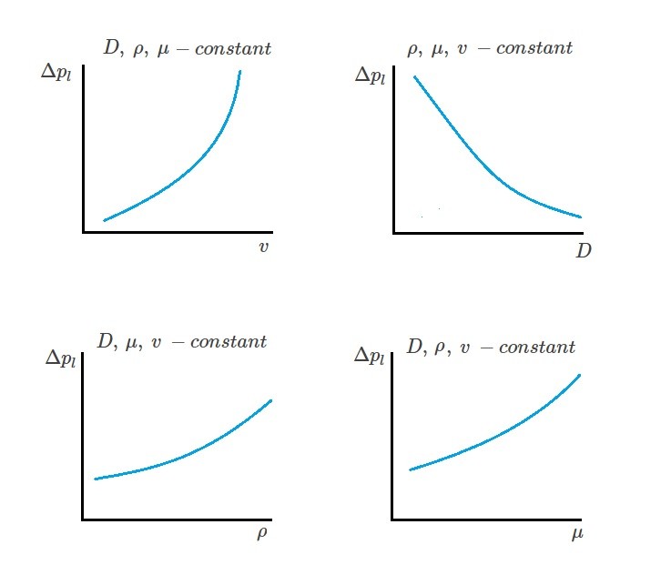
This data will only be valid for a specific pipe size and fluid that was used during the experiment. As a result, we still haven’t derived a general formulation. One way to derive a general formulation would be to vary the other variables and repeat the experiment until their is a sufficient amount of data. However, this is easier said than done. For example how can you vary the fluid density while holding the viscosity of the fluid constant? In addition, even if we are able to graph all of the variables in relation to the pressure drop, how does this give us the general formulation? To overcome this problem we will need to use two non-dimensional combinations of variable.
Dimensionless Products
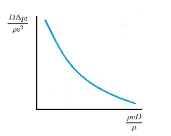
In turn, this will result in what is called dimensionless product or dimensionless groups. For a steady state, incompressible Newtonian fluid flowing through a straight horizontal pipe with a constant diameter the following equation will result.
(Eq 2) $\frac{DΔp_l}{ρv^2}=Φ\left(\frac{ρvD}{μ}\right)$
By taking this approach there will only be two variables instead of five that we need to work with. Hence, to conduct the experiment we will only need to vary the dimensionless product $ρvD/μ$ to find $DΔp_l/ρv^2$. As a result, we will be able to represent all of the variables that can effect the pressure drop per unit length in one single, universal curve. This will result in a curve that is valid for any combination of pipe size or different fluid type.
However, in order to perform this type of experiment you will need to consider the dimensions of the variables involved. In order to do this you will need to look at the basic dimensions of the variables. These basic dimensions are, $M$, length, $L$, and time $T$. However, if we consider Newton second law which is $F=MLT^{-2}, than we can change the basic dimensions to force, $F$, length $L$, and time $T$. As a result the two sides of equation 2 expressed in basic dimensions is as follows.
Left side:
(Eq 3) $\frac{DΔp_l}{ρv^2}=\frac{L(F/L^3)}{(FL^{-4}T^2)(LT^{-1})^2}=F^0L^0T^0$
Right side:
(Eq 4) $\frac{ρvD}{μ}=\frac{(FL^{-4}T^2)(LT^{-1})(L)}{FL^{-2}T}=F^0L^0T^0$
By using basic dimensions I am showing that the both sides of equation 2 are dimensionless. In turn, this will allow the graph that equation 2 generates to be independent from the system of units. As a result, we have performed a dimensional analysis. Knowing how to perform a dimensional analysis is important since it is used in the Buckingham pi theorem described the next article.