Fluid Element, Kinematic Analysis

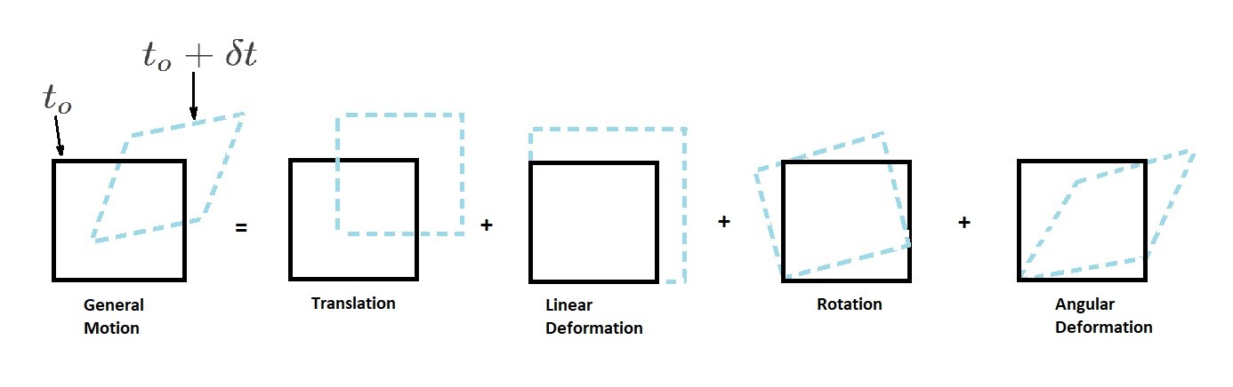
To start, let’s take a look at a fluid element and how to apply kinematics. For example, to start with, the fluid element will have a general motion.  General motion is made up of individual components.  These components are, translation, linear deformation, rotation, or angular deformation.  In addition, all of these components will be related to a time change $”\delta t”$.

Velocity and Acceleration Field

First, let’s review the velocity and acceleration fields.  First, the velocity field represents the velocity “$v$” at all point at all times within a specific area of interest. Hence, using a rectangular coordinate system, the velocity field will have the following notation, “$v(x,y,z,t)$”.  Where, x, y, z are directional coordinates and t is the time coordinate.  This notation represents the Eulerian method.

The velocity “$v$” is a vector quantity composing the three directional components x, y, and z.

(Eq 1)  $v=u\hat{i}+\nu \hat{j}+w\hat{k}$

In this equation $u$, $\nu$, and $w$ represent the velocity components in the x, y, and z directions.  In addition, $\hat{i}$, $\hat{j}$, and $\hat{k}$ are the corresponding unit vectors.  To further this, to perform a differential analysis, the velocity components will also have to depend on time.  As a result, if the velocity changes per unit time, than acceleration will occur.  The following equation will represent acceleration.

(Eq 2)  $a=\frac{\partial v}{\partial t}+u\frac{\partial v}{\partial x}+\nu \frac{\partial v}{\partial y}+w\frac{\partial v}{\partial z}$

This can further be broken down into the following scalar components.

$a_x=\frac{\partial u}{\partial t}+u\frac{\partial u}{\partial x}+\nu \frac{\partial u}{\partial y}+w\frac{\partial u}{\partial z}$

$a_y=\frac{\partial \nu }{\partial t}+u\frac{\partial \nu }{\partial x}+\nu \frac{\partial \nu }{\partial y}+w\frac{\partial \nu }{\partial z}$

$a_z=\frac{\partial w}{\partial t}+u\frac{\partial w}{\partial x}+\nu \frac{\partial w}{\partial y}+w\frac{\partial w}{\partial z}$

Acceleration can also be expressed concisely by using the following equation.

(Eq 3) $a=\frac{Dv}{Dt}$

To further this, the operator of the above equation is expressed as the following.

(Eq 4) $\frac{D()}{Dt}=\frac{\partial ()}{\partial t}+u\frac{\partial ()}{\partial x}+\nu \frac{\partial ()}{\partial y}+w\frac{\partial ()}{\partial z}$

Where, equation 4 is the material derivative.  The vector notation of the material derivative is as follows.

(Eq 5)  $\frac{D()}{Dt}=\frac{\partial ()}{\partial t}+(v·\nabla )()$

where

$\nabla ()=\frac{\partial ()}{\partial x}\hat{i}+\frac{\partial ()}{\partial y}\hat{j}+\frac{\partial ()}{\partial z}\hat{k}$

Linear Motion and Deformation

There are two basic type of motion; linear and angular.  First, let talk about linear motion of a fluid element.  For linear motion to occur, all physical points within the element must have the same velocity as the element moves from one point in time to another.  In other words there cannot be any velocity gradient across the fluid element.  However, velocity gradients are present.  Due this fact the fluid element will generally deform and rotate.

Let’s take a look at a small cube that has sides $\delta x$, $\delta y$, and $\delta z$ and a single velocity gradient of $\delta u/\delta x$.  For this example, we are going to have to refer to the image below.  As a result, from this image we can gather that x component for velocity between points B and O will be $u$.  On the other hand, the velocity between points C and A will be $u+\frac{\partial u}{\partial x}\partial x$.  The reason for the difference between velocity is due to “stretching” of the volume element.  The amount that volume element stretches is $\left(\frac{\partial u}{\partial x}\delta x\right)\partial t$.  Hence, OA stretches to OA’ and BC stretches to BC’.  As a result, the change in the original volume of the volume element is represented by the following equation.

(Eq 6) $changein\delta V=\left(\frac{\partial u}{\partial x}\delta x\right)(\delta y\delta z)(\delta t)$

In addition, the the rate of change of the volume “$\delta V$”  per unit volume in respect to the gradient $\partial u/\partial x$ is represented by the following equation.

(Eq 7) $\frac{1}{\delta V}\frac{d(\delta V)}{dt}=li{m}_{\delta t\to 0}\left[\frac{(\partial u/\partial x)\delta t}{\delta t}\right]=\frac{\partial u}{\partial x}$

Finally, if we were to include velocity  gradients $\frac{\partial \nu }{\partial y}$ and $\frac{\partial w}{\partial z}$, than equation 7 will be modified to the following equation.

(Eq 8)  $\frac{1}{V}\frac{d(\partial V)}{dt}=\frac{\partial u}{\partial x}+\frac{\partial \nu }{\partial y}+\frac{\partial w}{\partial z}=\nabla ·v$

This results in the volumetric dilatation rate which is the rate of change of the volume per unit volume.  Hence, we can conclude that as the element moves from one point to another, the fluid elements volume may change due to a velocity gradient.  However, if you are analyzing an incompressible fluid than the volumetric dilatation rate will be zero due to the fact the the fluid elements volume must remain constant.

 

Angular Motion and Deformation

In addition to linear motion, a fluid element can also experience angular motion.  For right now, let’s only focus on rotation on the x-y plane.

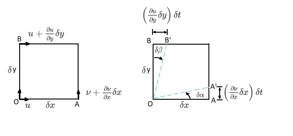
Let’s take a look at the image above.  This image represent angular motion as well angular deformation of a fluid element.  Basically, what is occurring is a velocity variation is causing the fluid element to rotate and deform.  This rotation and deformation will occur on the line segments $OA$ and $OB$ in short time intervals $\delta t$.  As a result the fluid element will rotate to a position $O{A}^{\prime }$ and $O{B}^{\prime }$ through the angles $\delta \alpha$ and $\delta \beta$.  In turn, using the following limit, the angular velocity ${\varpi }_{OA}$ about the line $OA$ is determined.

(Eq 9) ${\varpi }_{OA}=li{m}_{\delta t\to o}\frac{\delta \alpha }{\delta t}$

Furthermore, for small angles of deformation, the following equation can be applied.

(Eq 10) $tan\delta \alpha \approx \delta \alpha =\frac{(\partial /\nu )\delta x\delta t}{\delta x}=\frac{\partial \nu }{\partial x}\delta t$

In turn, equation 9 will become the following.

(Eq 11)  ${\varpi }_{OA}=li{m}_{\delta t\to 0}\left[\frac{(\partial \nu /\partial x)\delta t}{\delta t}\right]=\frac{\partial \nu }{\partial x}$

$\frac{\partial \nu }{\partial x}$ is positive when ${\varpi }_{OA}$ is rotating in a clockwise direction.

Similarly, the angular velocity ${\varpi }_{OB}$  for the line $OB$ can be determined using the same steps that were used to determine ${\varpi }_{OA}$.  In turn, for small angles of deformation, the following equation would be used to determine ${\varpi }_{OB}$.

(Eq 12) ${\varpi }_{OB}=li{m}_{\delta t\to 0}\left[\frac{(\partial u/\partial y)\delta t}{\delta t}\right]=\frac{\partial u}{\partial y}$

Unlike $\frac{\partial \nu }{\partial x}$,  $\frac{\partial u}{\partial y}$ will be positive when ${\varpi }_{OB}$ is rotating in a counter clockwise direction.  Using what we know about ${\varpi }_{OA}$ and ${\varpi }_{OB}$, we can determine the rotation, ${\varpi }_z$, about the z-axis.  Where, ${\varpi }_z$ is the average of ${\varpi }_{OA}$ and ${\varpi }_{OB}$.  Hence, if a counter-clockwise rotation is positive, than ${\varpi }_z$ will be the following.

(Eq 13) ${\varpi }_z=\frac{1}{2}(\frac{\partial \nu }{\partial x}-\frac{\partial u}{\partial y})$

In addition, the angular velocity around the x and y axes can be found in a similar manner. This will result in the following two equations.

(Eq 14) ${\varpi }_x=\frac{1}{2}(\frac{\partial w}{\partial y}-\frac{\partial \nu }{\partial z})$

and

(Eq 15) ${\varpi }_y=\frac{1}{2}(\frac{\partial u}{\partial z}-\frac{\partial w}{\partial x})$

By combining equation 13-15 the rotation vector, $\varpi$, can be found.

(Eq 16)  $\varpi ={\varpi }_x\hat{i}+{\varpi }_y\hat{j}+{\varpi }_z\hat{k}$

Finally, in addition, the rotation vector is also equal to half curl of the velocity vector.

(Eq 17)  $\varpi =\frac{1}{2}curlv=\frac{1}{2}\nabla \times v$

 

Previous | Next

⇑ | ⇓