In a system, the mass $M$, will remain constant as the system moves through the flow field. In other words, $\frac{DM_{sys}}{Dt}=0$. One way to analyze the mass in a system is by using a control volume. In turn, this will result in the continuity equation $\frac{∂}{∂t}\int{_{CV}}ρdV+\int{_{CS}}ρv·\hat{n}dA=0$. Using this method, however, will only allow you to analyze fluid that passes through the control surface of the control volume. As a result, it will not consider the fluid inside the control volume. Contrarily, to analyze the fluid inside the control volume you will need to obtain the differential form of the continuity equation.
Differential Form of the Continuity Equation
To derive the differential form of the continuity equation let’s take a look at a small, stationary cubical element. This element in essence will represent the control volume. At the center of element there will be a fluid density $ρ$, and the velocity coordinate components $u$, $ν$, and $w$. Due to the fact the fluid element is small, we will be able to define a volume integral.
(Eq 1) $\frac{∂}{∂t}\int{_{CV}}ρdV≈\frac{∂ρ}{∂t}δxδyδz$
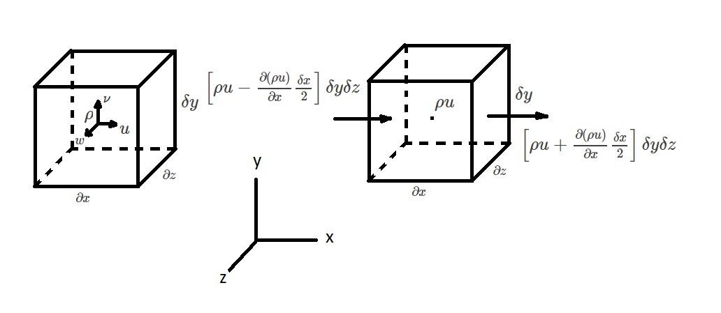
In addition to the volume integral, we will also need to show the rate of mass flow through the surface of the fluid element. To accomplish this, each coordinate direction will be defined separately. For example, let’s take a look at the x-direction. For the figure above, the mass rate of flow through the right face will represented by the following equation.
(Eq 2) $ρu|_{x+(δx/2)} = ρu+\frac{∂(ρu)}{∂x}\frac{δx}{2}$
The next equation will represent the rate of flow moving through the left face of the fluid element.
(Eq 3) $ρu|_{x-(δx/2)} = ρu-\frac{∂(ρu)}{∂x}\frac{δx}{2}$
Taylor series expansion of $ρu$ is used to derive equations 2 and 3. However, higher order terms were neglected. Next, these equations are multiplied by the the area $δyδz$. By doing this we will be able to define the net rate of mass out flow through the element.
(Eq 4) $Net~rate~of~mass~outflow~x~direction$$~=\left[ρu+\frac{∂(ρu)}{∂x}\frac{δx}{2}\right]δyδz-\left[ρu-\frac{∂(ρu)}{∂x}\frac{δx}{2}\right]δyδz$$~=\frac{∂(ρu)}{∂x}δxδyδz$
In addition, we will also want to define the mas out flow for both the y and z directions. The process used above will allow us to do this.
(Eq 5) $Net~rate~of~mass~outflow~y~direction$$~=\frac{∂(ρν)}{∂y}δxδyδz$
and
(Eq 6) $Net~rate~of~mass~outflow~z~direction$$~=\frac{∂(ρw)}{∂z}δxδyδz$
Next, combining equations 4 – 6 will derive the total net rate of mass outflow.
(Eq 7) $Net~rate~of~mass~outflow$$~=\left[\frac{∂(ρu)}{∂x}+\frac{∂(ρν)}{∂y}+\frac{∂(ρw)}{∂z}\right]δxδyδz$
Finally, the differential equation for conservation of mass is derived after combining the continuity equation of a control volume with equations 1 and 7.
(Eq 8) $\frac{∂ρ}{∂t}+\frac{∂(ρu)}{∂x}+\frac{∂(ρν)}{∂y}+\frac{∂(ρw)}{∂z}=0$
The conservation of mass or continuity equation is one of the fundamental equation of fluid mechanics. As a result, it will work for steady and unsteady flow. In addition, it will also work for both compressible and incompressible fluids.