In a previous article I talked about plane potential flows. These flows are governed by Laplace’s equations which are partial differential equations. As a result they can only be used for irrotational flows. However, Laplace’s equations will allow you to find various basic velocity potentials as wells as stream functions. In turn, using the method of superposition, these basic solutions can be combined to find more complex solutions. For this article I will focus on the superposition of a source and a uniform flow, which in turn will allow us to determine the flow around a half body.
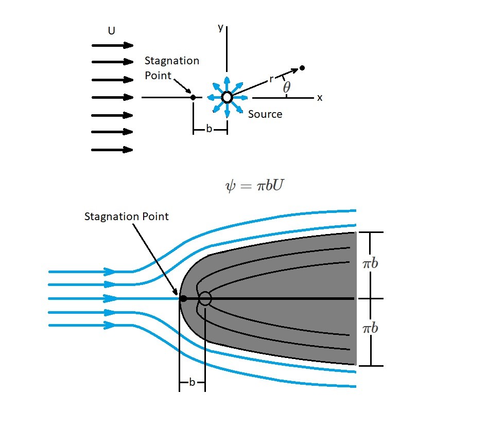
The image above shows a combination of a uniform flow and a source. When these two plane potential flows are superimposed an approximate representation of a flow around a half body will result. As a result, the stream function can be seen below.
(Eq 1) $ψ=ψ_{uniform~flow}+ψ_{source}=Ur~sin~θ+\frac{m}{2π}θ$
In addition, the following equation represents the velocity potential.
(Eq 2) $Φ=Ur~cos~θ+\frac{m}{2π}~ln~r$
Stagnation Point
In the above image a half body is shown. As the flow approaches the stagnation point the fluid velocity for the uniform flow will cancel out. Due to this, the fluid velocity will only be influenced by the source. Hence, to determine the velocity of the source you will need to use the following equation.
(Eq 3) $v_r=\frac{m}{2πr}$
Hence when $x=-b$, than $U$ will be determined by the following equation.
(Eq 4) $U=\frac{m}{2πb}$
Next, in order to determine what the stream function will be at the stagnation point $ψ$, the flow will need to be evaluated at $r=b$ and $θ=π$. As a result, the following equation is the stream function at the stagnation point.
(Eq 5) $ψ_{stagnation}=\frac{m}{2}$
Finally, taking in consideration that $m/2=πbU$ the equation of the streamline through the stagnation point will be the following.
(Eq 6) $πbU=Ur~sin~θ+bUθ$
or
(Eq 7) $r=\frac{b(π-θ)}{sin~θ}$
Where $θ$ is between $0$ and $2π$.
Half Body
Superimposing a uniform flow and a source will allow us to determine the streamlines of a fluid moving around a half body. In turn, the streamlines can be seen on the second picture of the image above. It is called a half body because the body is open at the down stream end. If you look at the image you will also notice that there are streamlines inside the the half body. In addition, to those stream lines the source is also within the half body. As a result, those streamlines are of no interest since we are only interested in the flow around the half body. However, they need to be noted to show how the source is used help define the streamlines flowing around the half body.
When we are looking at the width of half body it asymptotically approached $2πb$. As a result, the width of the half body is determined by the following equation.
(Eq 8) $y=b(π-θ)$
For the above equation, the half-widths $θ→0$ and $θ→2π$ approach $±bπ$.
Next, since the stream function is known, the velocity component at any point can be determined. As a result the velocity equations will be the following.
(Eq 9) $ν_r=\frac{1}{r}\frac{∂ψ}{∂θ}=U~cos~θ+\frac{m}{2πr}$
and
(Eq 10) $ν_θ=-\frac{∂ψ}{∂r}=-U~sin~θ$
Hence, the square of the velocity magnitude will be the following.
(Eq 11) $v^2=ν_r^2+ν_θ^2=U^2+\frac{Um~cos~θ}{πr}+\left(\frac{m}{2πr}\right)^2$
In addition, since $b=m/2πU$ equation 11 will become the following.
(Eq 12) $v^2=U^2\left(1+2\frac{b}{r}~cos~θ+\frac{b^2}{r^2}\right)$
Now that the velocity is known, the pressure at any point can be determined by using the Bernoulli equation. The Bernoulli equation is used to determine the difference in the flow field between two points. At the first point the pressure will be $p_o$ and the velocity will be $U$. While, at the second point the pressure will be $p$ and the velocity $v$. Hence,
(Eq 13) $p_o+\frac{1}{2}ρU^2=p+\frac{1}{2}ρv^2$