Plane potential flows allows us to approximate the streamlines of a fluid flow. It does this by using Laplace’s equations to determine the basic velocity potentials and stream functions for simple irrotational flows. In turn, these basic velocity potentials and stream functions are combined to determine the streamlines of more complex flows. This was shown for flow over a half body in the previous article. However, a half body is only a partial result showing how the flow behaves when it first encounters a body. In order to see how the flow would behave going over a complete body a Rankine oval would needs to be used.
First, when we looked at a half body we combined a uniform flow with a source. However, in order to determine the flow around a closed body we will need to add a sink. In turn, this will create a doublet between the source and the sink. For this article the source and the sink will have equal strength. For this type of situation the following stream function “$ψ$” and velocity potential “$Φ$” will be used.
( Eq 1) $ψ=Ur~sin~θ-\frac{m}{2π}(θ_1-θ_2)$
(Eq 2) $Φ=Ur~cos~θ-\frac{m}{2π}(ln~r_1-ln~r_2)$
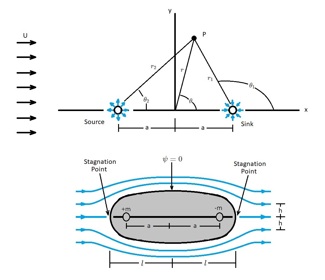
The image above visually represents the flow over a Rankine oval. As mentioned earlier, in order to solve this type of problem, you use a doublet combined with a uniform flow. In turn, the stream function can be written as the following.
(Eq 3) $ψ=Ur~sin~θ-\frac{m}{2π}~tan^{-1}~\left(\frac{2ar~sin~θ}{r^2-a^2}\right)$
or
(Eq 4) $ψ=Uy-\frac{m}{2π}~tan^{-1}~\left(\frac{2ay}{x^2+y^2-a^2}\right)$
In order to obtain a streamline $ψ$ will need to be set to a constant. As a result, if $ψ=0$ than a closed body will form. This is seen in the image above. In turn, the flow that is emanating from the sources is flowing into the sink. The oval shape that results is called a Rankine oval.
Half Length and Half Width
When analyzing a Rankine oval there will be two stagnation points. One stagnation point is caused by the sources, while the other is caused by the sink. In turn, the stagnation points will occur where the uniform velocity, source velocity, and sink velocity combine to equal a zero velocity. As a result the location of the stagnation points will be depend on the values of $a$, $m$, and $U$. Determining where the stagnation points are will allow you to define the body half-length $l$. To find the body half length the following equations will be used.
(Eq 5) $l=\left(\frac{ma}{πU}+a^2\right)^{1/2}$
or
(Eq 6) $\frac{l}{a}=\left(\frac{ma}{πUa}+1\right)^{1/2}$
Next, the body half-width $h$ of the Rankine oval needs to be determined. For the figure above, this is found by determining the value of $y$ where the y-axis intersect the $ψ=0$ streamline. Thus, for $ψ=0$, $x=0$ and $y=h$ the body’s half width is determined using the following equations.
(Eq 7) $h=\frac{h^2-a^2}{2a}~tan~\frac{2πUh}{m}$
or
(Eq 8) $\frac{h}{a}=\frac{1}{2}\left[\left(\frac{h}{a}\right)^2-1\right]~tan~\left[2\left(\frac{πUa}{m}\right)\frac{h}{a}\right]$
In turn, both the half-length and half-width are functions of the dimensionless parameter $πUa/m$. Hence, a large variety of body shapes that have different length to width ratios can be determined through different values of $Ua/m$. As a result, larger values of $Ua/m$ will result in a long slender body, while small values will result in a blunt shape.
Finally, when you are looking a Rankine oval, the surface pressure will increase with distance along the surface from the point downstream from the maximum body width. This is known as an adversed pressure gradient. In turn, this will typically result in a flow separation from the surface resulting in large low pressure wake. However, when the potential theory is used separation is not predicted. Hence, Rankine ovals will only provide a reasonable approximation outside the viscous boundary layer.