Plane potential flows describe the velocity gradient of a scalar function. In other words, it is describing the velocity potential. To do this the plane potential flow has to be an irrotational flow. As a result, this will allow us to make approximations for several different applications.
Plane potential flows are characterized by Laplace’s equation. Laplace’s equation is a linear partial differential equation. As a result, simple solutions can be used to find complex solutions. For example, $Φ_1(x,y,z)$ and $Φ_2(x,y,z)$ are both solutions to Laplace’s equation. Combining these solutions will result in $Φ_3$ where $Φ_3=Φ_1+Φ_2$.
For this article I will only be discussing two-dimensional flows. The following equation represents the velocity components for the Cartesian coordinate system.
(Eq 1) $u=\frac{∂Φ}{∂x}$, $ν=\frac{∂Φ}{∂y}$
In turn, The following equation represents the velocity components for the cylindrical coordinates system.
(Eq 2) $ν_r=\frac{∂Φ}{∂r}$, $ν_θ=\frac{1}{r}\frac{∂Φ}{∂θ}$
These equations, in turn, will allow us to define the following plane flow stream functions.
(Eq 3) $u=\frac{∂ψ}{∂y}$, $ν=-\frac{∂ψ}{∂x}$
and
(Eq 4) $ν_r=\frac{1}{r}\frac{∂ψ}{∂θ}$, $ν_θ=-\frac{∂ψ}{∂r}$
By defining the velocity equations as stream function the conservation of mass will have been satisfied. As a result, we will now be able to impose the irrotationallity condition, $\frac{∂u}{∂y} = \frac{∂ν}{∂x}$. This, in turn, can be applied to the stream functions.
(Eq 5) $\frac{∂}{∂y}\left(\frac{∂ψ}{∂y}\right)=\frac{∂}{∂x}\left(-\frac{∂ψ}{∂x}\right)$
or
(Eq 6) $\frac{∂^2ψ}{∂x^2}+\frac{∂^2ψ}{∂y^2}=0$
We can either use a stream function or a velocity potential for plane irrotational flow. However, for both cases, Laplace’s equation must be satisfied in two dimensions. The stream functions and velocity are potential are related. This was shown by the fact that lines of $ψ$ are streamlines, which is determined by this equation.
(Eq 7) $\frac{dy}{dx}|_{along~ψ=constant}=\frac{ν}{u}$
In turn, if we were to move from one point (x,y) to another point (x+dx, y+dy), than the change in $Φ$ is given by this relationship.
(Eq 8) $dΦ = \frac{∂Φ}{∂x}dx+\frac{∂Φ}{∂y}dy=udx+νdy$
Finally, the following is true along a line of constant for $Φ$ where $dΦ=0$.
(Eq 9) $\frac{dy}{dx}|_{along~Φ=constant}=-\frac{u}{ν}$
Next, comparing equation 7 to equation 9 the following conclusion is drawn. The line of constant $Φ$ (equipotential lines) are orthogonal to the line of constant $ψ$ at the point where they intersect. When we are looking at a potential flow field, a family of equipotential lines and streamlines will allow us to determine a flow net. This in turn will give us a tool to visualize flow patterns.
Uniform Flow
One of the simplistic plane potential flows is uniform flow. In turn, the streamlines of a uniform flow are all straight and parallel. As a result, the velocity is constant. In order to further understand uniform flow, take a look at the following image.
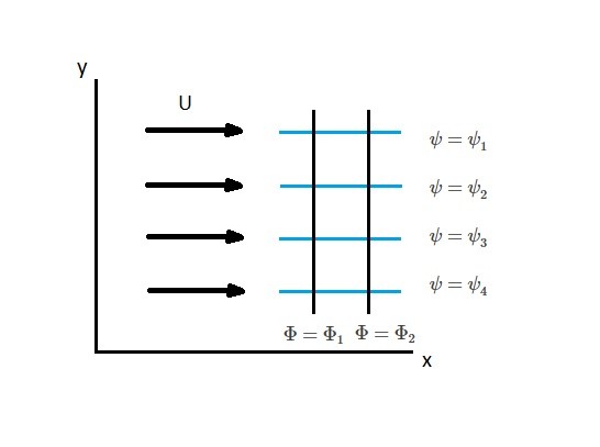
For the above image, the velocity potential is as follows.
(Eq 10) $\frac{∂Φ}{∂x}=U$, $\frac{∂Φ}{∂y}=0$
In turn, integrating these two equations will result in the following.
(Eq 11) $Φ=Ux+C$
Furthermore, $C$ is an arbitrary constant. As a result, $C$ can equal zero resulting in equation 11 become the following.
(Eq 12) $Φ=Ux$
In addition, similar manner is used to find the stream function.
(Eq 13) $\frac{∂ψ}{∂y}=U$, $\frac{∂ψ}{∂x}=0$
Thus, the stream function will become the following.
(Eq 14) $ψ=Uy$
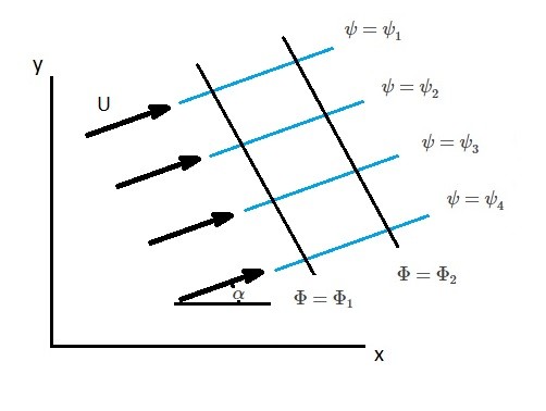
As well as flow moving solely in the x or y direction, it can also be offset by an angle $α$. Hence, a generalized form of the velocity potential and stream function will result.
(Eq 15) $Φ=U(x~cos~α+y~sin~α)$
(Eq 16) $ψ=U(y~cos~α-x~sin~α)$
Source and Sink
Sources and sinks are mathematical singularities within a flow field. Due to this fact, sources and sinks do not exist in real flow fields. However, when they are combined with other plane potential flows, they can be used to make an approximation for a real flow field. First, take a look at the image below.
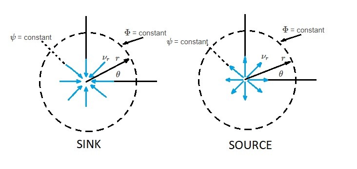
From this image we can see that for a sink the fluid will flow radially inward towards a singularity. On the other hand, a source has fluid flowing radially outward from a singularity. If we were to express this mathematically, we would first have to take a look at the volume flow rate $m$.
(Eq 17) $(2πr)ν_r=m$ or $ν_r=\frac{m}{2πr}$
Also, it should be noted that since the flow is purely radial than $ν_θ=0$. As a result, the velocity potential is derived by integrating these equations.
(Eq 18) $\frac{∂Φ}{∂r}=\frac{m}{2πr}$, $\frac{1}{r}\frac{∂Φ}{∂θ}$
Hence,
(Eq 19) $Φ=\frac{m}{2π}ln~r$
For equation 19 if $m$ is positive than the flow is coming from a source. Contrary, if $m$ is negative than the flow going towards a sink. For both a sink and a source, when $r=0$ than the velocity becomes infinite at the singularity. In reality this is impossible. However, as mentioned earlier, sources and sinks represent a hypothetical flow.
Next, we need to determine the stream function for a source and a sink through integration.
(Eq 20) $ν_r=\frac{1}{r}\frac{∂ψ}{∂θ}=\frac{m}{2πr}$ and $ν_θ=-\frac{∂ψ}{∂r}=0$
In turn, this yields:
(Eq 21) $ψ=\frac{m}{2π}θ$
From equations 19 and 21 it can be concluded that the streamlines, $ψ$, are radial line, while the equipotential lines, $Φ$, are concentric circles that are centered at the origin.
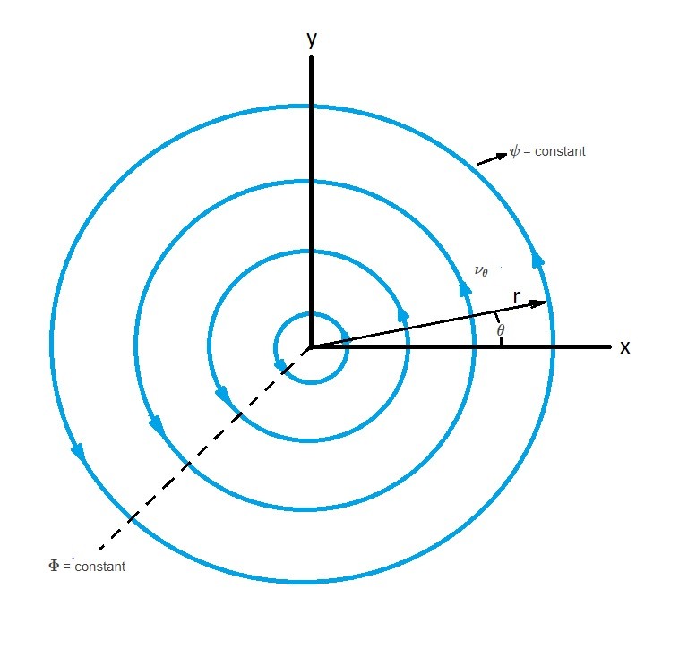
Vortex
Another plane potential flow is when the streamlines are in concentric circle. In other words, when the streamlines form a vortex. First, the velocity potential is as follows.
(Eq 22) $Φ=Kθ$
$K$ is a constant
Next, following equation represents the stream function.
(Eq 23) $ψ=-K~ln~r$
Since the streamlines are in a concentric circle $ν_r=0$ and
(Eq 24) $ν_θ=\frac{1}{r}\frac{∂Φ}{∂θ}=-\frac{∂ψ}{∂r}=\frac{K}{r}$
As a result, this equation indicates that the tangential velocity will vary inversely based off distance from the origin. This means that velocity will be infinite at $r=0$ creating a singularity.
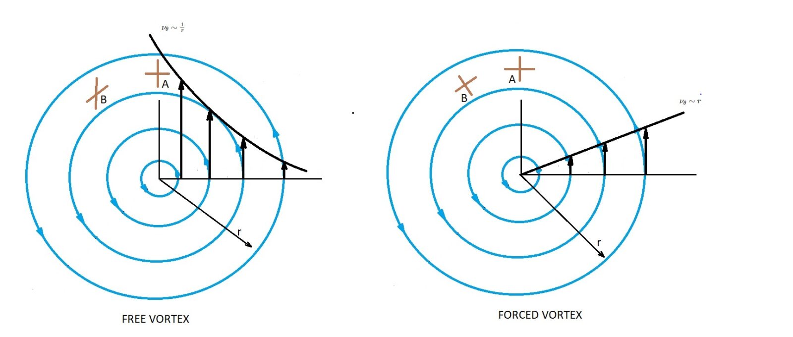
Vortex motion is an irrotational flow. This is because rotation is based of the orientation of the fluid instead of the path followed by the element. This, in turn, results in a free vortex. For example, take look at two sticks placed inside a free vortex. At point A, one stick is aligned to the streamline while the other is perpendicular. As the sticks move to point B, the stick that is aligned to the streamline will follow a circular path. However, the stick that is perpendicular to the streamline will rotate in a clockwise rotation due to the free vortex.
On the other hand, if the vortex were to rotate like a rigid body, than both sticks would rotate with the rigid body. This is a forced vortex, and unlike a free vortex, the flow is not irrotational. Due to this fact, a velocity potential cannot be used to describe the flow of a forced vortex. The image below shows an example of both a free and a forced vortex.
If you were to combine both a free and a forced vortex than a combined vortex will result. For a combined vortex, the center of the vortex will be a forced vortex while the outside will be a free vortex. The resulting velocity equations will be as follows.
(Eq 25) $ν_θ = ϖr~~r≤r_o$
(Eq 26) $ν_θ = \frac{K}{r}~~r>r_o$
$r_o$ = radius of central core
Vortex Circulation
Circulation “$Γ$” is a mathematical concept used to describe vortex motion. In order to determine circulation you will need to take the line integral of the tangential velocity around a closed curve in the flow field.
(Eq 27) $\oint{_C}v·ds$
As seen in the above equation, the integration will be performed around a closed curve “C”. In addition, this integration will be performed in the counter-clockwise direction where $ds$ is the differential length along the curve. When the flow is irrotational than $v=∇Φ$. In turn, $v·ds=∇Φ·ds=dΦ$. Hence, the following statement can be made for irrotational flow.
(Eq 28) $Γ=\oint{_C}dΦ$
In other words, if the flow is irrotational than the circulation will generally be zero. When the singularity is enclosed within the curve of circulation this statement may not be true.
This is the case for free vortex if $ν_θ=K/r$. In this case the circulation could occur around the circular path of the radius $r$. In turn, the following equation will result.
(Eq 29) $Γ=\int{_0^{2π}}\frac{K}{r}(r~dθ)=2πK$
Finally, to find the velocity potential and stream function of a free vortex use the following equations.
(Eq 30) $Φ=\frac{Γ}{2π}θ$
and
(Eq 31) $ψ=-\frac{Γ}{2π}ln~r$
This will help you evaluate forces acting on a body that is immersed in moving fluid.
Doublet
The final plane potential flow that I am going to discuss is the doublet. A doublet will result after combining a source and a sink.
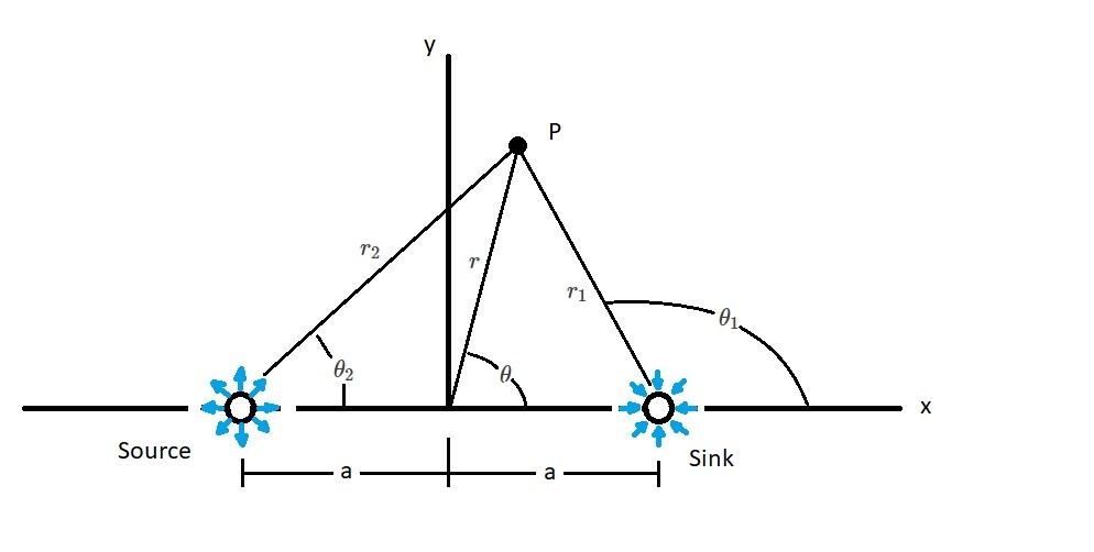
In the picture above, the source and sink will have equal strength. The following equation represents the stream function.
(Eq 32) $ψ=-\frac{m}{2π}(θ_1-θ_2)$
Next, we will rewrite equation 32 into the following.
(Eq 33) $tan~\left(-\frac{2πψ}{m}\right)=tan~(θ_1-θ_2) = \frac{tan~θ_1-tan~θ_2}{1+tan~θ_1~tan~θ_2}$
From the above figure the following is true.
(Eq 34) $tan~θ_1=\frac{r~sin~θ}{r~cos~θ-a}$
and
(Eq 35) $tan~θ_2=\frac{r~sin~θ}{r~cos~θ+a}$
Taking equation 34 and 35 into consideration equation 33 can be rewritten.
(Eq 36) $ψ=-\frac{m}{2π}~tan^{-1}~\left(\frac{2ar~sin~θ}{r^2-a^2}\right)$
If distance “$a$” can be considered small, allowing the value of the angle to considered a small angle, than the following equation can be used for the stream function.
(Eq 37) $ψ=-\frac{mar~sin~θ}{π(r^2-a^2)}$
A doublet is formed when the source and sink approach each other $(a→0)$ and the strength of $m$ increases $(m→∞)$ allowing the product of $ma/π$ remain constant. For the above equations $r/(r^2-a^2)→1/r$ which in turn allows equation 37 to reduce to the following equation.
(Eq 38) $ψ=-\frac{K~sin~θ}{r}$
$K=ma/π$
In turn the velocity potential for the doublet will be the following.
(Eq 39) $Φ=\frac{K~cos~θ}{r}$
The following image represents the streamlines for a doublet. It can be seen that the streamlines are circles that are going through an origin that is tangent to the x-axis.
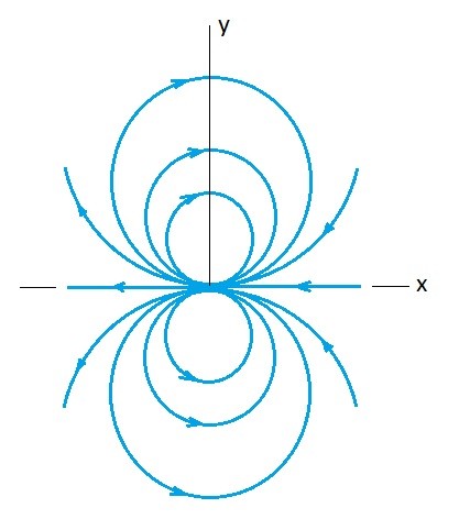
In reality doublets are not physically realistic entities. However, when doublets are combined with other plane potential flows than we can estimate a realistic flow.