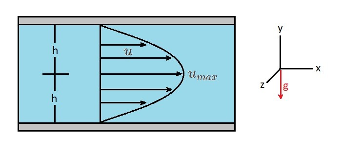
In a previous article I discussed the Navier-Stokes Equations. Using these equations, we can determine the flow between two fixed horizontal, infinite parallel plates. In order to to this, we will need to describe how the fluid particles move. For this case, there will be no flow in the y or z direction; $ν=0$ and $w=0$. As a result, all of the fluid flow will be in the x-direction. Hence, the resulting continuity equation will be $∂u/∂x=0$. In addition, $u$ will have no variation in the z-direction for the infinite plates. This means that the stead flow $∂u/∂t=0$ so that $u=u(y)$. Taking these conditions into account the Navier-Stokes equation will be reduced the following equations.
(Eq 1) $0=-\frac{∂p}{∂x}+μ\left(\frac{∂^2u}{∂y^2}\right)$
(Eq 2) $0=-\frac{∂p}{∂y}-ρg$
(Eq 3) $0=-\frac{∂p}{∂z}$
In these equations, $g_x=0$, $g_y=-g$, and $g_z=0$. As a result, the y-axis will point up.
Next, we will integrate equation 2 and 3 to generate the following equation.
(Eq 4) $p=-ρgy+f_1(x)$
In turn, this shows that there is a variation of pressure hydrostatically in the y-direction.
Next, equation 1 will be rewritten into the following form and integrated twice.
(Eq 5) $\frac{d^2u}{dy^2}=\frac{1}{μ}\frac{∂p}{∂x}$
First integration:
(Eq 6) $\frac{du}{dy}=\frac{1}{μ}\left(\frac{∂p}{∂x}\right)y+c_1$
Second integration:
(Eq 7) $u=\frac{1}{2μ}\left(\frac{∂p}{∂x}\right)y^2+c_1y+c_2$
Now that the integration has been performed the two constants $c_1$ and $c_2$ will need to be determined. In order to do this you will first need to apply boundary conditions. In this case I have already said that the plates are fixed. Hence, $u=0$ for $y=±h$, which will satisfy the no slip condition for a viscous fluid. As a result the two constants for a fixed condition will become the following.
(Eq 8) $c_1=0$
and
(Eq 9) $c_2=-\frac{1}{2μ}\left(\frac{∂p}{∂x}\right)h^2$
Now that $c_1$ and $c_2$ have been defined, the velocity distribution can be fully derived.
(Eq 10) $u=\frac{1}{2μ}\left(\frac{∂p}{∂x}\right)(y^2-h^2)$
In turn, the resulting velocity profile between the fixed plates is parabolic.
Volume Rate of Flow
The volume flow rate ,$q$, represents the total volume of fluid pass between the two plates. As a result, to determine the volume flow rate you need to define a unit width $a$ along with total distance, $2h$, between the plates. Mathematically, the volume flow rate is obtained through the following relationship.
(Eq 11) $q=\int{^h_{-h}}u~dy=\int{^h_{-h}}~\frac{1}{2μ}\left(\frac{∂p}{∂x}\right)(y^2-h^2)dy$$=-\frac{2h^3}{3μ}\left(\frac{∂p}{∂x}\right)$
Due to the fact that the pressure will decrease in the direction of the flow, the pressure gradient $∂p/∂x$ will negative. As a result, if $Δp$ is the pressure drop between two points separated by the distance $l$.
(Eq 12) $\frac{Δp}{l}=-\frac{∂p}{∂x}$
Applying equation 12 to equation 11 will allow us to express the volume flow rate as the following.
(Eq 13) $q=\frac{2h^3Δp}{3μl}$
In turn, taking in consideration that the pressure gradient is inversely proportional to the viscosity and has a strong dependence on the gap width, the mean velocity can be determined.
(Eq 14) $v=\frac{q}{2h}=\frac{h^2Δp}{3μl}$
Finally, maximum velocity will occur at $y=0$ between the two the parallel plates. As a result, the maximum velocity can be expressed in the following mathematical form.
(Eq 15) $u_{max}=-\frac{h^2}{2μ}\left(\frac{∂p}{∂x}\right)=\frac{3}{2}v$