To understand Prandtl Boundary Layer you will have to have an understanding of the Navier Stokes equations. This is because for any flow that is viscous and incompressible the governing Navier Stokes equations can be used to define the fluids boundary layer as it flows past a submerged object. As a result, the equations below are the Navier Stokes equations for a steady, two dimensional laminar flow that has negligible gravitational effects.
(Eq 1) $u\frac{∂u}{∂x}+v\frac{∂u}{∂y}=-\frac{1}{ρ}\frac{∂p}{∂x}+ν\left(\frac{∂^2u}{∂^2u∂x^2}+\frac{∂^2u}{∂^2u∂y^2}\right)$
(Eq 2) $u\frac{∂u}{∂x}+v\frac{∂u}{∂y}=-\frac{1}{ρ}\frac{∂p}{∂x}+ν\left(\frac{∂^2u}{∂^2u∂x^2}+\frac{∂^2u}{∂^2u∂y^2}\right)$
$ρ$ = fluid density
$ν$ = kinematic viscosity
The above equations are an expression of Newtons second law. In addition, the conservation of mass equation for an incompressible flow is as follows.
(Eq 3) $\frac{∂u}{∂x}+\frac{∂v}{∂y}=0$
Prandtl Boundary Layer
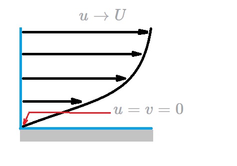
The mathematical conditions needed to define a boundary layer are well known. At a certain distance away from the body the fluids velocity will be the same as the upstream velocity. On the other hand the fluid making contact with body will stick to the body causing it to have a zero velocity. Despite the fact that the boundary conditions are well known, currently no one has obtained an analytical solution. However, there are approximations, and that is where Prandtl Boundary layer comes in.
Prandtl was able to derive certain approximations that made it possible to simplify the governing equations. From these simplified equations one of Prandtl’s students, H. Blasius, solved these simplified equations to find the boundary layer of a fluid flowing over a flat plate. First, due to the fact that the boundary layer is thin, it can be expected that a velocity normal to the plane will be much smaller than if it were parallel to the plate. As a result, the rate of change of any parameter across the boundary layer should be significantly greater than along the flow direction. Hence,
(Eq 4) $v<<u$ and $\frac{∂}{∂x}<<\frac{∂}{∂y}$
This means that physically, the flow is parallel to the flat plate. As a result, any fluid property will be distributed downstream faster than it would across the streamlines. In turn this will allow the Navier Stokes equations, as well as the conservation of mass equation, to reduce to the following boundary layer equations.
(Eq 5) $\frac{∂u}{∂x}+\frac{∂v}{∂y}=0$
(Eq 6) $u\frac{∂u}{∂x}+v\frac{∂u}{∂y}=v\frac{∂^2u}{∂y^2}$
Like the Navier Stokes equations, these boundary layer equations are non-linear partial differential equations. However, there are differences between the two. For instance, the y momentum equation is not included. Instead the continuity equation is left unaltered while the x momentum equation is modified. In addition, the pressure variable has been removed. As a result, the velocity variable in the x and y direction are the only unknowns. This is because the pressure for a flat plate is constant through out the pressure field. Hence the flow will be a balance between the viscous and inertial forces where pressure has no role. This will result in the following boundary conditions for the governing boundary layer equations.
(Eq 7) $u=v=0$ at $y=0$
(Eq 8) $u→U$ as $y→∞$
Dimensionless Form
It can be stated that regardless of the location along the plate the dimensionless form of the boundary layer velocity profile on a flat plate should be similar.
Or,
(Eq 9) $\frac{u}{U}=g\left(\frac{y}{δ}\right)$
In the above equation $g(y/δ)$ is an unknown function that will need to be determined. In addition, the boundary layer thickness is inversely proportional to square root of $U$. This is determined by applying an order of magnitude analysis of the forces that are acting only the fluid.
(Eq 10) $δ∼\left(\frac{νx}{U}\right)^{1/2}$
These conclusions are based off the balance between the viscous and inertial forces within the boundary layer. In addition, the the fact the velocity will vary more rapidly in the direction across the boundary layer than along it must also be considered. As a result, the dimensionless similarity variable is derived.
(Eq 11) $η=\left(\frac{U}{νx}\right)^{1/2}y$
In addition, the stream function is the following.
(Eq 12) $ψ=(νxU)^{1/2}f(η)$ where $f=f(η)$
Finally, for a 2-dimensional flow the stream function is $u=∂ψ/∂y$ and $v=-∂ψ/∂x$. For the flow over a flat plate these general equations become the following.
(Eq 13) $u=Uf'(η)$
and
(Eq 14) $v=\left(\frac{νU}{4x}\right)^{1/2}(ηf’-f)$
Next, when equations 13 and 14 are substituted into the two governing equations 5 and 6 a third-order ordinary differential equation will result.
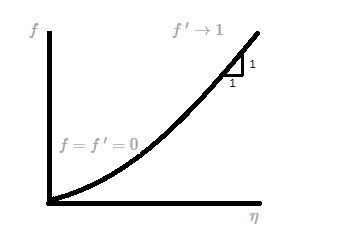
(Eq 15a) $2f~”’+ff~”=0$
The boundary conditions for this equation will be as follows.
(Eq 15b) $f=f~’=0$ at $η=0$ and $f~’→1$ as $η→∞$
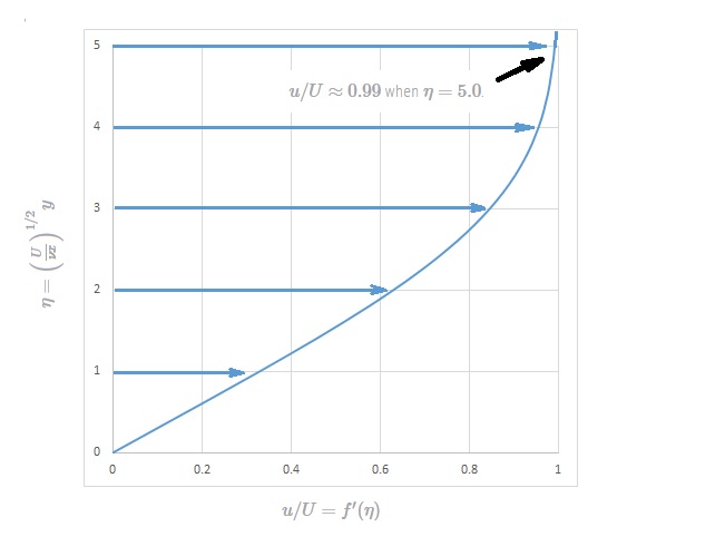
Even though equation 15 does not provide an analytical solution it can be easily integrated using a computer. The dimensionless boundary layer profile, $u/U=f'(η)$ is shown in the following figures and tabulated in the following table. It is termed the Blasius solution.
Blasius Solution
| $η=y(U/νx)^(1/2)$ | $f'(η)=u/U$ |
| 0 | 0 |
| 0.4 | 0.1328 |
| 0.8 | 0.2647 |
| 1.2 | 0.3938 |
| 1.6 | 0.5168 |
| 2 | 0.6298 |
| 2.4 | 0.729 |
| 2.8 | 0.8115 |
| 3.2 | 0.8761 |
| 3.6 | 0.9233 |
| 4 | 0.9555 |
| 4.4 | 0.9759 |
| 4.8 | 0.9878 |
| 5 | 0.9916 |
| 5.2 | 0.9943 |
| 5.6 | 0.9975 |
| 6 | 0.999 |
From the Blasius Solution $u/U≈0.99$ when $η=5.0$. As a result,
(Eq 16) $δ=5\sqrt{\frac{νx}{U}}$ or $\frac{ð}{x}=\frac{5}{\sqrt{Re_x}}$
In addition, the displacement, $δ^*$, and momentum, $Θ$, are found using the following equations.
(Eq 17) $\frac{δ^*}{x}=\frac{1.721}{\sqrt{Re_x}}$
and
(Eq 18) $\frac{Θ}{x}=\frac{0.664}{\sqrt{Re_x}}$
Finally, the wall shear stress can be obtained using the following equation.
(Eq 19) $τ_w=0.332U^{3/2}\sqrt{\frac{ρμ}{x}}$