One of the main aspects of boundary layer theory is to determine the drag caused by the shear forces acting on a body. One method of accomplishing this is by using the momentum integral boundary layer equation. Throughout this article I will be considering a uniform flow over a flat plate. The pressure will be assumed to be constant throughout the flow field. In addition, the flow entering the control volume, which will be stationary, will be uniform. However, the flow exiting the control volume will vary from the upstream velocity. This means that the velocity at the edge of the boundary layer will be approximately the same as the upstream velocity. On the other hand, the fluid velocity on the plate will be zero.
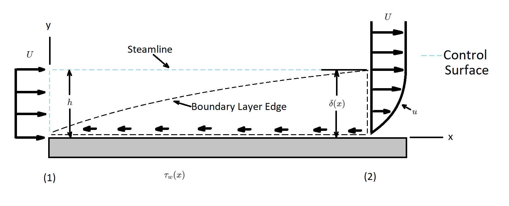
In the image above the fluid that is adjacent to the plate will make up the lower portion of the control surface. On the other hand, the upper surface will coincide with streamline that is just outside of the control volume.
Momentum Equation
Before we get started let’s take a look at the general linear momentum equation.
(Eq 1) $\frac{∂}{∂t}\int{_{cv}}vρV+\int{_{cs}}vρv·\hat{n}dA=\sum{F_{cv}}$
$v$ = velocity
$ρ$ = density
$V$ = volume
$A$ = cross-sectional area
First, we are going to apply the x-component to the momentum equation.
(Eq 2) $\sum{F_x}=ρ\int{_{(1)}}uv·\hat{n}dA+ρ\int{_{(2)}}uv·\hat{n}dA$
Next, to determine the drag, $D$, on the flat plate plate we will need to input the plates width, $b$, into the above equation.
(Eq 3) $\sum{F_x}=-D=-\int{_{plate}}~τ_w~dA=-b\int{_{plate}}~τ_w~dx$
Note, that the net force is caused by the uniform pressure contribution. It, however, does not contribute to the flow. As a result, since the plate is solid, and the upper surface of the control volume is streamline, there will be no flow through this area in the control volume. Hence, equation 3 will become the following.
(Eq 4) $-D=ρ\int{_{(1)}}U(-U)dA+ρ\int{_{(2)}}u^2dA$
or
$D=ρU^2bh-ρb\int{^δ_0}~u^2~dy$
In the above equations the height is not known. However, by the conservation of mass the flowrate through section 1 must equal the flowrate through section 2. As result,
(Eq 5) $Uh=\int{^δ_0}~u~dy$
Equation 5 can also be written as the following.
(Eq 6) $ρU^2bh=ρb\int{^δ_0}~Uu~dy$
Next equation 4 and 6 are combined to determine the momentum flux across outlet of the control volume.
(Eq 7) $D=ρb\int{^δ_0}~u(U-u)~dy$
If the flow were inviscid than the drag would be zero. As a result the shear stress would also be zero. In reality this is not case. In stead there is a balance between the shear / drag (left-hand side equation 7) and the decrease in momentum (right-hand side of equation 7). What this means if $x$ increase $δ$ increases, which in turn causes the drag to increase. Hence, the boundary layer must thicken to overcome drag. Due to this fact drag can also be written in the terms of the momentum thickness $Θ$.
(Eq 8) $D=ρbU^2Θ$
This equation is valid for both laminar and turbulent flows.
Next, by differentiating both sides of equation 8 in respect to x we can determine the shear stress contribution.
(Eq 9) $\frac{dD}{dx}=ρbU^2\frac{dΘ}{dx}$
Since $dD=τ_wbdx$ we can derive the following equation.
(Eq 10) $\frac{dD}{dx}=bτ_w$
Momentum Integral Boundary Layer Equation
Finally, by combining equations 9 and 10 we will be able to derive momentum integral boundary layer equation.
(Eq 11) $τ_w=ρU^2\frac{dΘ}{dx}$
This equation gives as the ability to obtain reasonable drag and shear stress results even when the velocity profile isn’t completely accurate.
Now let’s consider a general velocity profile.
(Eq 12) $\frac{u}{U}=g(Y)$ for $0≤Y≤1$ and $\frac{u}{U}$ for $Y>1$
where $Y=y/δ$ varies from 0 to 1 across the boundary layer.
In this equation, the dimensionless function $g(y)$ can be any shape of interest. However, it should be a reasonable approximation of the boundary layer profile for accurate results. In addition, the boundary conditions $u=0$ at $y=0$ and $u=U$ at $y=δ$ must be satisfied. Or,
$g(0)=0$ and $g(1) = 1$
Next, equation 7 is used to determine the drag.
(Eq 13) $D=ρb\int{^δ_0}u(U-u)dy$$=ρbU^2δ\int{^1_0}g(Y)[1-g(Y)]dY$$=ρbU^2δC_1$
In addition, the wall shear stress is the following.
(Eq 14) $τ_w=μ\frac{∂u}{∂y}|_{y=0}$$\frac{μU}{δ}\frac{dg}{dY}|_{Y=0}=\frac{μU}{δ}C_2$
Equations 13 and 14 are than combined.
(Eq 15) $δdδ=\frac{μC_2}{ρUC_1}dx$
Next, equation 15 is integrated from $δ=0$ at $x=0$.
(Eq 16) $δ=\sqrt{\frac{2νC_2x}{UC_1}}$ or $\frac{δ}{x}=\frac{\sqrt{2C_2/C_1}}{Re_x}$
Taking this into consideration equation 14 will become the following.
(Eq 17) $τ_w=\sqrt{\frac{C_1C_2}{2}}U^{3/2}\sqrt{\frac{ρμ}{x}}$
Finally, the constants $C_1$ and $C_2$ need to be determined. These can by determine from the local friction coefficient $c_f$ and the friction drag coefficient $C_{Df}$.
(Eq 18) $c_f=\frac{\sqrt{2C_1C_2}}{\sqrt{Re_x}}$
$Re$ = Reynolds Number
(Eq 19) $C_{Df}=\frac{\sqrt{8C_1C_2}}{\sqrt{Re_l}}$
The local friction coefficient and the friction drag coefficient are dependent on the laminar flow velocity profile. The table below can be used for common velocity profiles.
|
Profile Character |
$δ\sqrt{Re_x}/x$ |
$c_f\sqrt{Re_x}$ |
$C_{Df}\sqrt{Re_L}$ |
|
Blasius Solution |
5.00 |
0.664 |
1.328 |
|
Linear $u/U=y/δ$ |
3.46 |
0.578 |
1.156 |
|
Parabolic $u/U=2y/δ-(y/δ)^2$ |
5.48 |
0.730 |
1.460 |
|
Cubic $u/U=3(y/δ)/2$$-(y/δ)^3/2$ |
4.64 |
0.646 |
1.292 |
|
Sine Wave $u/U=sin[π(y/δ)/2]$ |
4.79 |
0.655 |
1.310 |