For a problem to be multi loading it means that the problem would have forces on in it in different directions. This would in turn cause different stresses on the part in different direction. These stresses could be both normal and shear stresses. First let’s look at a problem that only has normal stresses on it. Refer to the problem below.

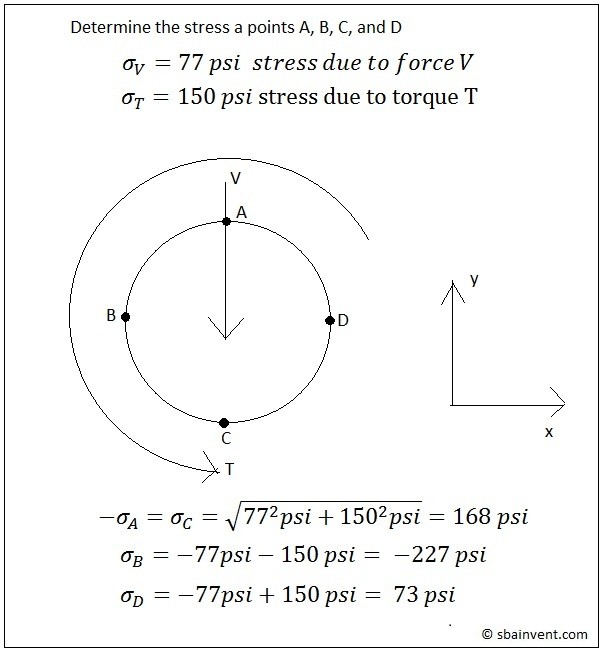
The same concepts apply to problems that consist of shear forces; refer to the problem below.
Stress Elements
Elements are used to express the different stress on the points that were shown above in a more simplified manner. They will show both the normal stresses and shear stresses on one diagram. To view what a stress element looks like refer to the figure below.
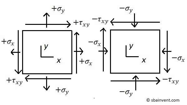
For three dimensional problems there can be up to three of these elements representing the xy, xz, and yz faces.
Principle Stresses, & Maximum Shear Stress
The principle stresses are the maximum and minimum normal stress that are caused by the applied stresses. On a graph they will represent the maximum points on the x-axis. This will be discussed further when talking about Mohr’s circle. To calculate the principle stresses for a 2d problem equation 1 would be used.
(Eq 1) $σ_{1,2} = \frac{σ_x+σ_y}{2}\pm\sqrt{\left(\frac{σ_x-σ_y}{2}\right)^2+τ_{xy}^2}=σ_{avg}\pmτ_{max}$
$σ$ = Normal Stress
$τ$ = Shear Stress
The part before the plus and minus sign of equation 1 is the average normal stress, equation 2.
(Eq 2) $σ_{avg} = \frac{σ_x+σ_y}{2}$
In addition to calculating the principle stresses, the maximum shear stress can be calculated. To calculate the maximum shear stress you would used the part after the plus and minus sign of equation 1, refer to equation 3.
(Eq 3) $τ_{max} = \sqrt{\left(\frac{σ_x-σ_y}{2}\right)^2+τ_{xy}^2}$
To calculate the graphical angle of the shear stress in respect to the normal stress equation 4 would be used.
(Eq 4) $\tan(2θ_p)=\frac{τ_{xy}}{(σ_x-σ_y)/2}$
2d Mohr’s Circle
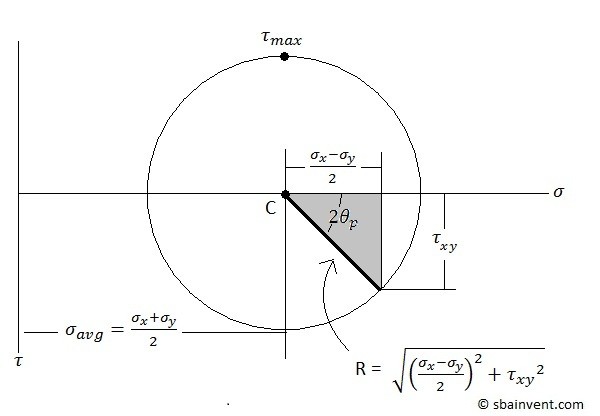
The 2d Mohr’s circle is a graphical representation of the equations seen above. To view a 2d graphical Mohr’s circle refer to the figure below.
3d Mohr’s Circle
The 3d Mohr’s circle is developed by the same methods as the 2d Mohr’s circle except there are 2 additional shear stresses to consider, and one more principle stress to consider. To solve for the principle stresses for a 3d problem the roots of equation 5 would have to be determined. Also, equations 6 thru 8 would have to be used to solve equation 5.
(Eq 5) $σ^3-I_1σ^2+I_2σ-I_3=0$
(Eq 6) $I_1=σ_x+σ_y+σ_3$
(Eq 7) $I_2 = σ_xσ_y + σ_xσ_z + σ_yσ_z – τ_{xy}^2 – τ_{xz}^2 – τ_{yz}^2$
(Eq 8) $I_3 =\left|\begin{matrix} σ_x & τ_{xy} & τ_{xz}\cr τ_{xy} & σ_y & τ_{yz} \cr τ_{xz} & τ_{yz} & σ_z \end{matrix}\right|$
$σ$ = Normal Stress
$τ$ = Shear Stress
Equation 8 is a 3X3 determinant. If you’re not sure how to solve a determinant follow this link.
To solve for the maximum shear stresses equation 9 would be used.
(Eq 9) $ τ_{1,2,3}=\frac{σ_1-σ_2}{2}~or~\frac{σ_1-σ_3}{2}~or~\frac{σ_2-σ_3}{2}$
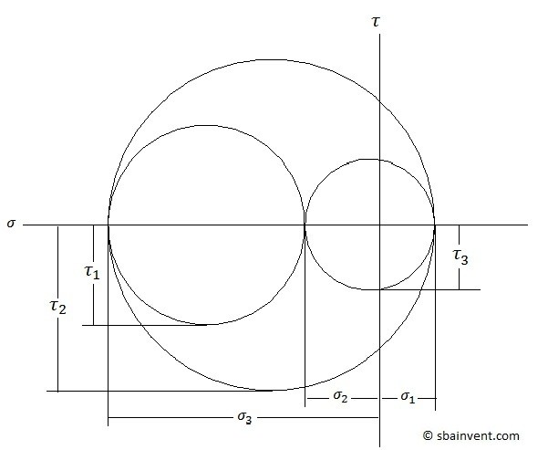
Refer to the figure below to derive a 3d Mohr’s Circle from equations 5-9.
Maximum Stress Criteria
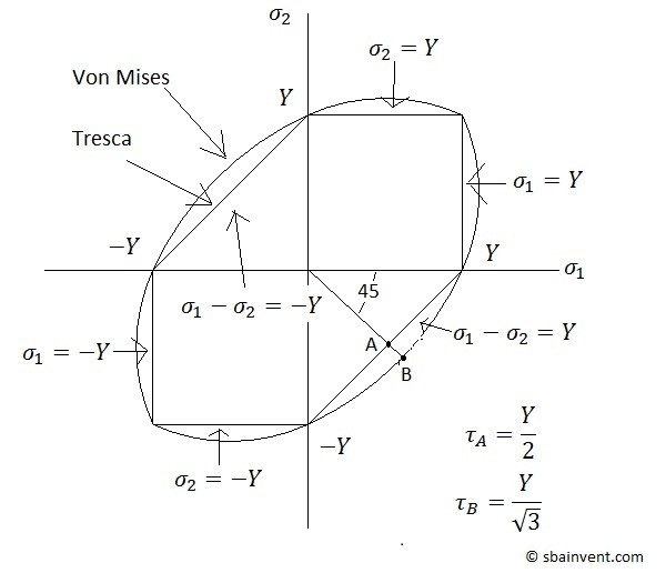
There are different stress criterions implemented to determine if a part is going to yield when it has stress on it in different directions. The two that I’m going to discuss are the Tresca stress criteria and the Von Mises stress criteria.
Both criterions relate the principle stresses to the yield stress of the material in question. The Tresca Stress criteria represents the maximum stress as a hexagon in principle stress space. Due to this, the Tresca Stress criteria is typically more conservative when it comes to shear stress, and sometimes the materials can take a stress that is 15% higher than the stress predicted by Tresca. Von Mises on the other hand does not take a conservative approach. To view both the Tresca and Von Mises plot in principle stress space refer to the figure below.
Stress to Strain Conversion
It is also possible to calculate strain in one direction when there is stresses in multiple directions by using equations 10-15.
(Eq 10) $ε_x=\frac{1}{E}(σ_x-νσ_y-νσ_z)$
$ε$ = Normal Strain
$σ$ = Normal Stress
$E$ = Youngs Modulus
$ν$ = Poissons Ratio
(Eq 11) $ε_y = \frac{1}{E}(σ_y-νσ_x-νσ_z)$
(Eq 12) $ε_z = \frac{1}{E}(σ_z-νσ_x-νσ_y)$
(Eq 13) $ϒ_{xy} = \frac{1}{2G}τ_{xy} = \frac{1+ν}{E}τ_{xy}$
$γ$ = Shear Strain
$τ$ = Shear Stress
$G$ = Shear Modulus
(Eq 14) $γ_{xz} = \frac{1}{2G}τ_{xz}=\frac{1+ν}{E}τ_{xz}$
(Eq 15) $γ_{yz} = \frac{1}{2G}τ_{yz}=\frac{1+ν}{E}τ_{yz}$
The same principles discussed here will apply when calculating strains in multiple directions.