Fatigue Stress

Up to this point static failure has been the main point of discussion. However, it is possible for a part to fail at lower load then what was originally expected when that load is applied to the specimen in a cyclical manner. This is known as fatigue failure. Typically it takes thousands to millions of cycles before fatigue failure occurs. However, you can experience a fatigue failure by bending a paper clip back and forth. Of course this happens a lot faster than most fatigue failures, and that is because you are permanently deforming the paper clip after each bend which you wouldn’t want to happen in a real application.

Phases of Fatigue Failure

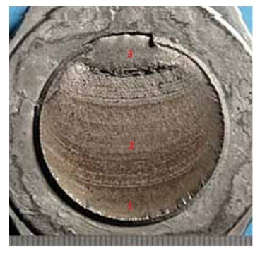
The appearance of a fatigue failure is very similar to what a brittle fracture would look like. It however happens in phases, and because of this fatigue failure will normally happen unexpectedly. Also, it is important to note that different conditions such as stress concentrations can cause fatigue failure to occur faster than expected. A list of the phases can be seen below.

1. The first phase is introduction of micro-cracks due to the cyclic plastic deformation. These micro-cracks cannot be seen by the human eye, but continue to form as loading is applied then removed in a cyclical manner.
2. The next phase is when the micro-cracks form into macro-cracks. These cracks will form a parallel plateau like fracture on its surface. This is commonly known as beach marks or clam shell marks.
3. Finally, as the macro-cracks continue to grow the specimen will finally not be able to support the load and a sudden fracture of the material will occur.

Refer the figure below to see how the fatigue failure will progress through a specimen.

S-N Diagrams

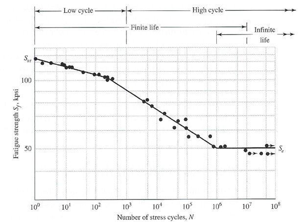
To help determine when a specimen will fail S-N diagrams are constructed to compare the fatigue strength (Sf) to the life cycle of the specimen N. For some materials, such as steel and iron, the S-N diagram will become horizontal at a certain point, this point is known as the endurance point S’e. Refer to the figure below for UNS G41300 steel.

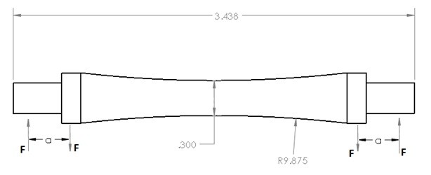
S-N diagrams are constructed in of data obtained off of specimens in a controlled laboratory environment. The specimens will have no geometric stress concentrations, and the surface will be highly polished to eliminate the potential of surface stresses. The test is normally a simple controlled bending test where the specimen is rotated at a specific speed so that the loading will fluctuate from a compressive load to a tensional load. Refer to the figure below to see the shape of a typical specimen that might be used.

 

Due to the fact that this is an experiment that is controlled it is possible that even if a part uses that exact material it most likely will not fail at the same time as specified by the S-N diagram. Instead the S-N diagram should be used as a guide. This is why it is important as an engineer to perform tests on a newly developed products to make sure everything is performing as expected.

Fatigue Limit

It is also possible to calculate the fatigue limit based on how many cycles you would want the specimen to endure before it fails. To do this equations 1 through 3 would be used.

(Eq 1)  $S_f=aN^b$

(Eq 2)  $a=\frac{(fS_{ut})^2}{S_e}$

(Eq 3)  $b=-\frac{1}{3}log\left(\frac{fS_{ut}}{S_e}\right)$

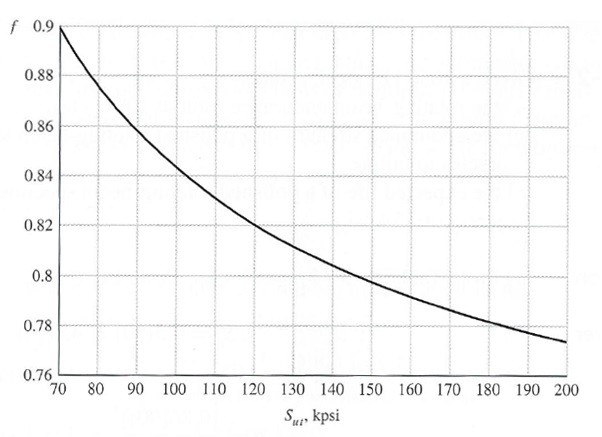
From equations S_ut represents the ultimate tensile strength, S_e represents the endurance limit, and f represents the fatigue strength fraction. The fatigue strength fraction can be found using the figure below.

Endurance Limit

When determining the fatigue limit there are number of factors that are normally considered. They are represented in the equation below.

(Eq 4)  $S_e=k_ak_bk_ck_dk_ek_fS’_e$

Where ka represents the surface condition modification factor, kb represents the size modification factor, kc represents the load modification factor, kd represents the temperature modification factor, ke represents the reliability factor, kf represents any other miscellaneous effects, and S’_e is the endurance limit determined during the rotary beam test used to create the S-N diagram. The reason why modification factors should be included instead of the just using the value obtained from test data is because the test data does not take in consideration of any variations that could occur to the specimen. The modification factors on the other hand can be used to improve the estimation of the endurance factor. The data obtained during testing can be used to represent the S’_e value, however, it is also acceptable to use the data seen in equation 5 for steel.

(Eq 5)   $S’_e=\cases{0.5S_{ut} & S_{ut}≤200kpsi(1400~MPa) \cr 100kpsi & S_{ut}>200~kpsi \cr 700~MPa & S_{ut}>14000MPa}   $

The surface factor will take in consideration a variety of different surface conditions. The reason why this is important is because for the beam testing the specimen is highly polished to remove any surface defects. If these surface defects are left, cracks are more likely to start at those points, which in effect will lower the overall endurance limit. Equation 6 and the table below would be used to determine the surface factor modification for different surface finishes on steel.

(Eq 6) $k_a = aS_{ut}^b$

Surface Finish	Factor a		Factor b
	$S_{ut}$, kpsi	$S_{ut}$, MPa
Ground	1.34	1.58	-0.085
Machined	2.70	4.51	-0.265

In addition the surface conditions the size of the specimen also needs to be considered. The reason for this is because as the size of a specimen increases the statistical imperfections in the sample. So as the size of the specimen increases, the endurance limit will start to decrease. The size factor needs to only be considered for bending and torsional loads. If the load is axial then the size factor can be set equal to 4. If it is the bending or torsional loading then equation 4 can be used to determine the size factor.

(Eq 7)  $k_b=\cases{(d/0.3)^{-0.107}  &  0.11≤d≤2in  \cr  0.91d^{-0.157} & 2<d≤10in \cr (d/7.62)^{-0.107} & 2.79≤51mm \cr 1.51d^{-0.157}  & 51<d≤254mm}$

Make note that the variable d in equation 7 represents the diameter of a rod. If the specimen happens to be rectangular the equation 8 could be used to compute an equivalent diameter.

(Eq 8)  $d_e=0.808(hb)^{1/2}$

S’_e is determined using a bending force on the test specimen. However there are different types of loads besides bending that can be place on the specimen, and these can affect the actual endurance limit. To determine what the load factor would be for bending, axial force, and a torsional force refer to equation 6.

(Eq 9)  $k_c = \cases {1 & bending \cr 0.85 & axial \cr 0.59 & torsion   }$

Testing is normally done at room temperature. However, it is known that temperature can change how a material is expected to behave. For example the lower the temperature the more brittle the material will normally become, while at higher temperatures that material will normally become more ductile. Temperature will also have an effect on the predicted endurance limit. The temperature factor is determined by taking a ratio of tensile strength at operating temperature (S_T) over the tensile strength at room temperature (S_RT).

(Eq 10)  $k_d = \frac{S_T}{S_{RT}}$

Refer to the table below to see the temperature factor for steel at different temperatures.

Temperature, $^oC$	$k_d$
20	1.000
150	1.025
300	0.975
450	0.843
600	0.549

 

The test data taken during testing will have some statistical variation between samples. Due to this statistical variation a reliability factor needs to be included to adjust the endurance limits according to how reliable you want your prediction to be. This is because the test endurance limit is essentially calculated by a best fit line through a scatter plot. To calculate the reliability faction equation 11 and the table below would be used.

(Eq 11)  $k_e = 1-0.08z_a$

Finally, there are miscellaneous effects that can affect the endurance limit. An example of a miscellaneous effect would be how a stress concentration would affect the sample. There are also other residual stresses that you may or may not know about that can affect the endurance limit. This is something that the engineer has to keep in mind even if he or she cannot determine what these values actually are, which is why safety factors are used.

Fatigue Example Problem

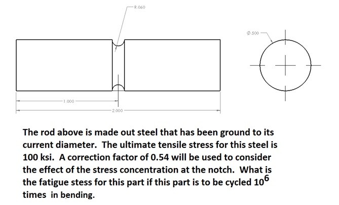
Answer

$S_f = aN^b$

$a=\frac{(fS{ut})^2}{S_e}$

$b=-\frac{1}{3}log\left(\frac{fS_{ut}}{S_e}\right)$

$f=0.843$

Determine $S_e$

$S_e=k_ak_bk_ck_dk_ek_fS’_e$

$S’e=0.5S_{ut}=0.5(100ksi)=50ksi$

$k_a=aS_{ut}^b=1.34(100)^{-0.085}=0.906$

$k_b=(d/0.3)^{-0.107}=(0.5/0.3)^{-0.107}=0.947

$k_c=1$ (Bending)

$k_d =1 $ (It is assumed that the part will be operating in a $20^oC$ environment since there is no information provided)

$k_e=1 -0.08(2.326)=0.814$ (Assumed 99% reliability, since it wasn’t noted you can make any assumption you want)

$k_f=0.54$

$S_e=(0.906)(0.947)(1)(1)(0.814)(.54)(50ksi)=18.87ksi$

Determine maximum fatigue stress

$a=\frac{(0.843(100ksi))^2}{18.87ksi}=376.6ksi$

$b=-\frac{1}{3}log\left(\frac{0.843(100ksi)}{18.87ksi}\right)=-0.217$

$S_f=376.6ksi(10^6)^{-0.217}=18.79ksi$