Turbulent flow, unlike laminar flow, has a chaotic and random behavior that effects multiple fluid parameters. In turn, this will effect the fluid velocity, shear stress, pressure, and fluid temperature. Basically, turbulent flow is three-dimensional vorticity problem. As a result, different terms will have there own mean value. For example the velocity $u=u(x,y,z,t)$ represents the x component of instantaneous velocity. However, for a turbulent flow we will need to find the time mean value $\bar{u}$. This done with the following equation.
(Eq 1) $\bar{u}=\frac{1}{T}\int{^{t_o+T}_{t_o}}~u(x,y,z,t)dt$
$T$ is a time interval that is considerably longer than the period of the longest fluctuation, but considerably shorter than the any unsteadiness within the average fluid velocity. $u’$ represents the fluctuating velocity. The fluctuation velocity is a time-varying portion that is different than the average velocity.
or
(Eq 2) $u=\bar{u}+u’$
Mathematically the average of the fluctuations is zero.
(Eq 3) $\bar{u’}=\frac{1}{T}\int{^{t_o+T}_{t_o}}~(u-\bar{u})~dt$$=\frac{1}{T}\left(\int{^{t_o+T}_{t_o}}~udt-\bar{u}\int{^{t_o+T}_{t_o}}~dt\right)$$=\frac{1}{T}(T\bar{u}-T\bar{u})=0$
Hence the fluctuations within the turbulent flow are equally distributed over the average. In addition, since the square of the fluctuation cannot be negative, the average value will always be positive. As a result,
(Eq 4) $\bar{(u’)^2}=\frac{1}{T}\int{^{t_o+T}_{t_o}}~(u’)^2dt>0$
Structure and Characteristics of Turbulent Flow Variation
Depending on the situation, the structure, as well as the characteristics, can vary from one situation to another. One example is turbulent intensity. The turbulent intensity is the level of turbulence. An example of when the turbulent intensity can vary is on windy day. If the wind is gusty the turbulent intensity will be greater than if the wind was steady. To find the turbulent intensity you would take the square root of the mean square of the fluctuating velocity over the time average velocity.
(Eq 5) $Þ=\frac{\sqrt{\bar{(u’)^2}}}{\bar{u}}=\frac{\left[\frac{1}{T}\int{^{t_o+T}_{t_o}}~(u’)^2~dt\right]^{1/2}}{\bar{u}}$
In addition for turbulent intensity the period of the fluctuation differs between one flow situation to another. The frequency of fluctuations can range from 10 to 1000 cycles per second just for water flowing through a faucet. On the other hand, if you were to look Gulf Stream current or the flow in atmosphere on one of the gas planets, the fluctuation period could occur from hours to days or possibly longer.
Shear Stress
To find the shear stress for a laminar flow you would use $τ=μ~du/dy$. It might be tempting to replace the instantaneous velocity $u$ with the time averaged velocity $\hat{u}$, this however will lead to inaccurate results. In other words for turbulent flow $τ≠μ~d\hat{u}/dy$.
To understand why the above is true, we first need to take a look at what laminar flow really is. For a laminar flow to occur the fluid particle will flow smoothly along layers that allow the particles to glide past one another, In other words the flow is not entirely random. Instead it can be easily tracked since a slight bias in one direction will produce a flowrate that can be associated with fluid particles motion $\hat{u}$. In addition, a momentum flux in the x-direction will create a drag on the fluid particles. This drag will create a shear stress on the particle which in turn causes particles to move slower the closer they are to the wall of a pipe.
Now let’s take a look at turbulent flow. For a turbulent flow the above a statement is also true. The main difference is that there is also random motion of individual fluid particles. Basically, there is also random, three-dimensional eddy type motion. This eddy type motion promotes mixing within the fluid, which is not present in a laminar flow. In turn, this greatly increases the x-momentum which will cause relatively large shear forces within the fluid. This means that the total shear forces is a combination of the laminar shear forces and the turbulent shear forces caused by the eddy type motion. The turbulent shear force will be a product of the x-velocity $u’$, the rate of mass transfer across the plane A-A $ν’$, and the fluid density. To find the total shear force you will need to use the following equation.
(Eq 6) $τ=μ\frac{d\bar{u}}{dy}-ρ\overline{u’ν’}=τ_{lam}+τ_{turb}$
If the flow were laminar than $u’=v’=0$. In turn, this would cause $\overline{u’v’}=0$. This means that for laminar flow $τ_{lam}=μd\bar{u}/dy$. On the other hand the turbulent shear stress $τ_{turb}=-ρ\overline{u’v’}$ is positive. As a result, the shear stress for turbulent flow will be greater than it is for laminar flow. In fact the shear stress for a turbulent flow can be 100 to 1000 times greater than it for laminar flow on the outer regions of the velocity profile.
In order to obtain accurate results for turbulent flow you will need to have accurate knowledge of what $τ_{turb}$. To do this you will need to know what the fluctuations of $u’$ and $v’$ are. This is because currently it has not been possible to solve the governing equations for turbulent flow using the Navier-Stokes equations. Instead numerical techniques are used which require powerful computers to solve.
Eddy Viscosity: Shear Stress
In addition to the equations in the above section, eddy viscosity, $η$ can be used to determine what the turbulent shear stress is.
(Eq 7) $τ_{turb}=η\frac{d\bar{u}}{dy}$
The eddy viscosity approach is an extension of the laminar flow terminology that was developed by J. Boussinesq. In practice this is not an easy parameter to use. The reason why is because eddy viscosity is a function of the fluid and the flow conditions instead of given value for the fluid like absolute viscosity. In other words, this value cannot be looked up in a handbook since it is unique to the turbulent flow condition. There are however, several semiempirical theories that can be used to approximate the eddy viscosity. One theory would be to view a turbulent process as a random transport of bundles of fluid particles over a certain distance $l_m$; which is the mixing length. Using this and apply some ad hoc assumption and approximation of the eddy viscosity can be found using the following equation.
(Eq 8) $η=ρl^2_m\left|\frac{d\bar{u}}{dy}\right|$
Hence, the shear stress can found using the following equation.
(Eq 9) $τ_{turb}=ρl^2_m\left(\frac{d\bar{u}}{dy}\right)^2$
However, to make the above work, you will now need to determine what the mixing length, $l_m$, is. This can be difficult since $l_m$ is not constant through the flow field. Due to this fact additional assumption, that can effect accuracy, will need to be made.
Turbulent Flow Velocity Profile
Based off the distance from wall of a pipe a fully developed turbulent flow can be broken down into three different regions. These regions are the viscous sub layer, which is very near the pipe wall, the overlap region, and the outer turbulent layer though the center portion of the flow. In the viscous sub layer the viscous shear stress is dominant while the turbulent and and random eddying nature of the flow is basically absent. On the other hand, in the outer turbulent layer the turbulent stress is dominant causing significant mixing and randomness of the flow. It can be seen that the characteristics of the flow between the viscous sub layer and outer turbulent layer are quite different. In the viscous sub layer the fluid viscosity is most important parameter, while fluid density doesn’t matter. In contrast for the outer turbulent layer the opposite is true.
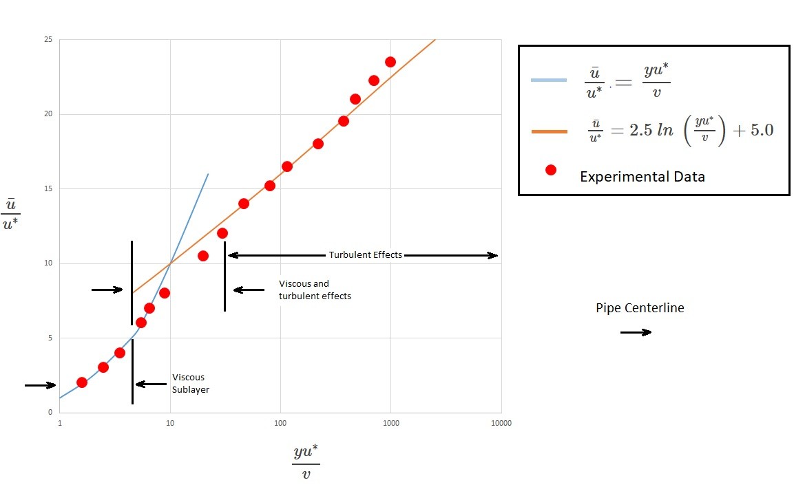
For the viscous sub layer it can be written in the following dimensionless form to represent this portion of the velocity profile.
(Eq 10) $\frac{\bar{u}}{u^*}=\frac{yu^*}{v}$
In this equation $y=R-r$. This is the distance measured from the wall. In addition, $\bar{u}$ is the time-average velocity in the x-direction. Finally, $u^*$ is the friction velocity. It can be found by using the following equation; $u^*=(τ_w/ρ)^{1/2}$.
Next, dimensional analysis shows that the overlap region will vary with the log of y. As a result, the following equation is used to define this region of the velocity profile.
(Eq 11) $\frac{\bar{u}}{u^*}=2.5~ln~\left(\frac{yu^*}{v}\right)+5.0$
The constants 2.5 and 5.0 in the above equation were determined experimentally. This equation will give a reasonable representation of the velocity profile in the area of flow that is not to close to the pipe wall but is also not way out in the center of the pipe. The following figure shows the velocity profile derived by equations 10 and 11 in comparison to experimental data. Note the horizontal scale is logarithmic which exaggerates the size of the viscous sub layer.
The following equation represents the central region of the pipe.
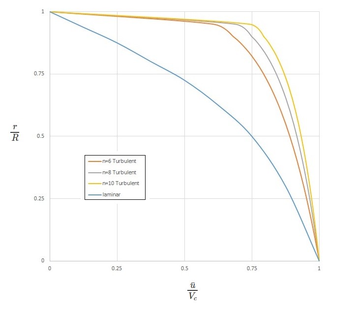
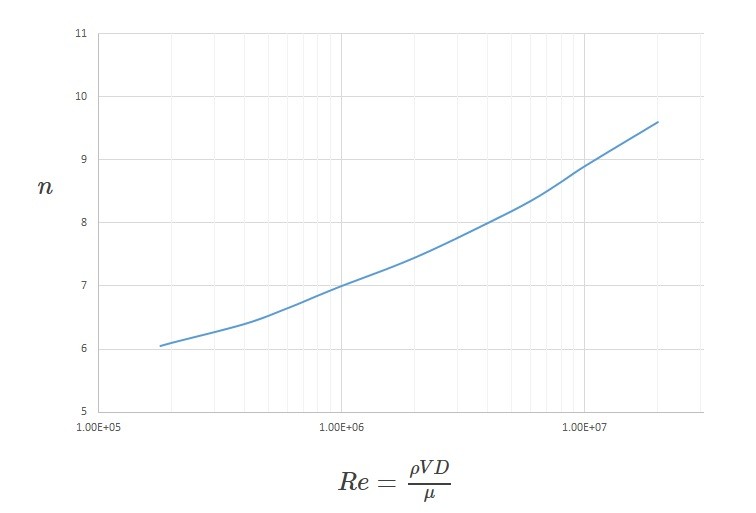
(Eq 12) $\frac{\bar{u}}{V_c}=\left(1-r/R\right)^{1/n}$
In this equation $V_c$ is the center line velocity of the flow. In addition, $n$ is a function of the Reynolds number. It can be determine from the following graph. This equation is not valid for flow that is close to the wall of the pipe.
The graph below shows typical laminar flow and turbulent flow velocity profiles derived from equation 12.