When a flow is fully developed it will have the same velocity profile at any cross-section within the pipe. This statement is true for both laminar flow and turbulent flow. However, the details of the two types of flows are very different.
Now why do we even care about the velocity profile? The main reason is because the velocity profile will provide us with key information to find other aspects of the flow. For example, by using the velocity profile the pressure drops, flow rates, and head loss can be determined.
Even though most flows are turbulent, for this article I will be focusing on laminar flow. It is important to learn the theory behind fully developed laminar flow because it is one the few viscous analysis that can be carried out without making assumptions and approximations. This in turn will give you the foundation to perform more complex analysis. There are three different analysis methods that can be used for fully developed laminar flow. They are applying Newton’s second law of motion directly to a fluid element, using Navier Stokes equations, or using dimensional analysis methods. For this article I will only being focusing on using Newton’s second law of motion.
Newton’s Second Law of Motion: Laminar Flow
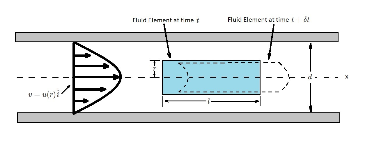
Newton’s second law states that force will equal mass times acceleration, or simply $F=ma$. To apply Newton’s second law, we will first look at a fluid element at a time $t$. Also, since fluid flow generally occurs in a round pipe, will need to consider the pipe length $l$, the pipe diameter $d$, and the radius $r$ of the fluid element. In addition, for right now everything will be analyzed in a horizontal pipe
The next step is to apply a time derivative $t+δt$ as the fluid moves to a new location. Also, it is important to realize that when the fluid first enters a pipe it is not fully developed. As a result, $t$ will become distorted at $t+δt$. However, once the fluid is fully developed this distortion will be same at the two different locations that are analyzed. In turn, the fluid will not be experiencing acceleration at any point in the fluid element for fully developed flow. As a result, the local acceleration will be zero or $δv/δt=0$. In addition, since the flow is fully developed, the convection acceleration will also be zero, or $v⋅∇v=u∂u/∂x\hat{i}=0$.
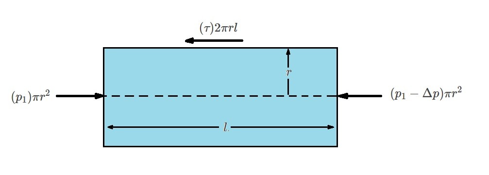
Next, since we are looking at a horizontal pipe the effects of gravity will be negligible. When this occurs the pressure will be constant across the vertical cross-section of the pipe. However, because of viscous effects it will vary from one section of the pipe to the next. Hence, mathematically this means that in section (1) $p=p_1$, but in section (2) it will become $p_2=p_1-Δp$. This shows that a pressure drop, $Δp$, has occurred due to a shear stress acting on the fluid. The shear stress is caused by the viscous effects of the fluid. In addition, it is a function of the pipe’s radius $τ=τ(r)$.
When a fluid become fully developed, a balance between pressure and viscous forces has occurred. The resulting equation represents this balance of forces.
(Eq 1) $(p_1)πr^2-(p_1-Δp)πr^2-(τ)2πrl=0$
or
$\frac{Δp}{l}=\frac{2τ}{r}$
Wall Shear Stress
Equation 1 provides us with a basic balance of the forces that are driving the fluid particles at a constant velocity. From this equation the shear stress can be derived. In order to do this you will need to take in account that neither $Δp$ or $l$ are a function of the radial coordinate $r$. As a result, $2τ/r$ is also independent of $r$. Because of this we can say that $τ=Cr$ where $C$ represents a constant. This means that when $r=0$ than there will be no shear stress. On the other hand at $r=d/2$ the shear stress will be at its maximum, where $τ_w$ is the wall shear stress. After taking these statements into this into consideration it can be concluded that $C=2τ_w/d$. Hence, the following equation is used to find the shear stress distributed throughout the pipe.
(Eq 2) $τ=\frac{2τ_wr}{d}$
In addition, the pressure drop and the shear stress are related through the following equation.
(Eq 3) $Δp=\frac{4lτ_w}{d}$
As a result, even if the shear the stress is small a large pressure drop can occur if the pipe is long.
Velocity Profile and Shear Stress
Equations 1-3 are valid for both laminar flow and turbulent flow. However, the way the shear stress and fluid velocity is related to one another is different for laminar flow and turbulent flow. This is because more assumptions are required to relate the shear stress to fluid velocity for turbulent flow than for laminar flow. As a result, turbulent flow is very complex. However, for laminar flow the shear stress is proportional to the velocity gradient $τ=μ~du/dy$. Hence, for pipe flow the velocity gradient will become the following equation.
(Eq 4) $τ=-μ\frac{du}{dr}$
This equation and equation 1 represent the governing laws for a fully developed laminar flow of a Newtonian fluid in a horizontal pipe. Equation 1 is Newton’s second law of motion while equation 4 is the definition of a Newtonian Fluid. Combining these two equations will result in the following.
$\frac{du}{dr}=-\left(\frac{Δp}{2μl}\right)r$
Next, integrating this equation will give use the velocity profile.
$u=-\left(\frac{Δp}{4μl}\right)r^2+C_1$
In this equation $C_1$ represents a constant. Now since the fluid will stick to the pipe wall due to viscosity we know that $u=0$ at $r=d/2$. As a result, $C_1=(Δp/16μl)d^2$. Taking this into consideration, the velocity profile will become the following.
(Eq 5) $u(r)=\left(\frac{Δpd^2}{16μl}\right)\left[1-\left(\frac{2r}{d}\right)^2\right]$$=v_c\left[1-\left(\frac{2r}{d}\right)^2\right]$
where $v_c$ is the centerline velocity.
Finally, an alternate expression of equation 6 can be written to relate the wall shear stress to the pressure gradient.
(Eq 6) $u(r)=\frac{τ_wd}{4μ}\left[1-\left(\frac{r}{R}\right)^2\right]$
$R=d/2$
Flowrate
When the velocity profile is plotted, a parabolic shape will result. The maximum velocity, $v_c$, will occur at the centerline of the pipe. On the other hand, the fluid velocity will be zero at the pipe walls. In order to obtain the flowrate of the velocity profile you will need to integrate the velocity profile across the pipe.
$Q=\int{u}~dA$$=\int{}^{r=R}_{r=0}u(r)2πr~dr$$=2πv_c~\int{}^R_0\left[1-\left(\frac{r}{R}\right)^2\right]r~dr$$=\frac{πR_2v_c}{2}$
Since $v_c=Δpd^2/(16μl)$ the above equation can be simplified to the following.
(Eq 7) $Q=\frac{πd^4Δp}{128μl}$
Finally, average velocity is found by dividing the flowrate by the cross-sectional area $v=Q/A$. Hence,
(Eq 8) $v=\frac{πR^2v_c}{2πR^2}=\frac{v_c}{2}=\frac{Δpd^2}{32μl}$
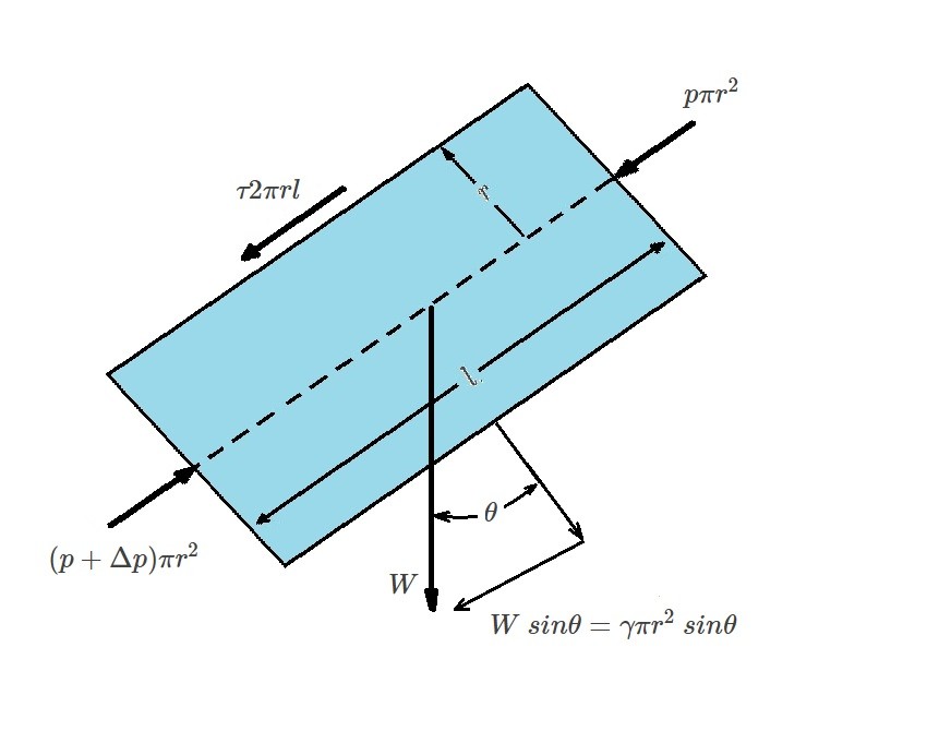
Non-Horizontal Pipes
Up to this point I have only talked about fully developed laminar flow in horizontal pipes. However, in a real life situations the pipe may not always be horizontal. This is easily remedied by replacing the pressure drop $Δp$ with $Δp-γl~sinθ$ in order to include the gravitational effects. Doing this will result in the following modified equations.
(Eq 9) $\frac{Δp-γl~sinθ}{l}=\frac{2τ}{r}$
(Eq 10) $v=\frac{(Δp-γl~sinθ)d^2}{32μl}$
and
(Eq 11) $Q=\frac{π(Δp-γl~sinθ)d^4}{128μl}$