When you are analyzing a fluid there could be several aspects that you could be interested in. For instance you might be interested in how a certain part of the fluid moves. On the other hand how the fluid flows over an object might be of interest. In addition how the fluid behaves in a certain volume of space might be of interest. The first aspect is an example of a system analysis. While the second and third requires a control volume. However, there could be cases where you need to consider both. In order to do this you will need to relate them to one another. This will require the use of the Reynolds transport theorem.
First, let’s take a look at the following equation.
(Eq 1) $B=mb$
In the above equation “B” represent various physical parameters. This could be velocity, acceleration, mass, temperature, or momentum. While “b” represents the amount of a physical parameter per unit mass. Finally, “m” represents the mass of the portion of fluid that is of interest. Refer to the table below as an example.
|
Physical Parameter |
B |
b=B/m |
|
mass |
$m$ |
$1$ |
|
momentum |
$mv$ |
$v$ |
|
kinetic energy |
$\frac{1}{2}mv^2$ |
$\frac{1}{2}v^2$ |
In equation 1 “B” is an extensive property, making it proportional to the amount of mass that is being considered. On the other hand “b” is an intensive property since it is independent of mass. Hence, when analyzing a system, $B_{sys}$ will represent the extensive property of the system. $B_{sys}$ will be determined by adding up the amount of the parameter of interest that is associated with each fluid particle of the system. As a result, $B_sys$ can be represented by the following limit where $δv→0$.
(Eq 2) $\lim_{δv\to 0}\sum_ib_i(ρ_iV_i)=\int{_{sys}}ρb~dV$
$ρ = density$
$V = volume$
The laws that govern fluid motion normally have time rate of change of an extensive property. As a result equation 2 would become the following.
(Eq 3) $\frac{dB_{sys}}{dt}=\frac{d(\int{_{sys}}ρb~dV)}{dt}$
Finally, equation 3 can also be used to represent a control volume as seen in the equation below.
(Eq 4) $\frac{dB_{CV}}{dt}=\frac{d(\int{_{CV}}ρb~dV)}{dt}$
Equations 3 and 4 may look similar, however they are mathematically different. They are mathematically different by the limits of integration. However, they are related by the Reynolds transport theorem. Due to this relationship there is a time rate of change between the extensive property of both the system and the control volume.
Deriving the Reynolds Transport Theorem
The purpose of the Reynolds transport theorem is to relate system concepts to control volume concepts. Let’s take a look at the image below. In this image we have a fixed control volume with a 1-dimensional flow. The control volume is between section 1 and 2. At current time $t$ the system that we will consider is within the specified control volume. However, after a short time $t+δt$, the system will move slight towards the right. As result the fluid particle that originally coincided in section II have moved to the right $δl_2=v_2δt$. Similarly, the fluid particles in section 1 have moved to the right $δl_1=v_1δt$.
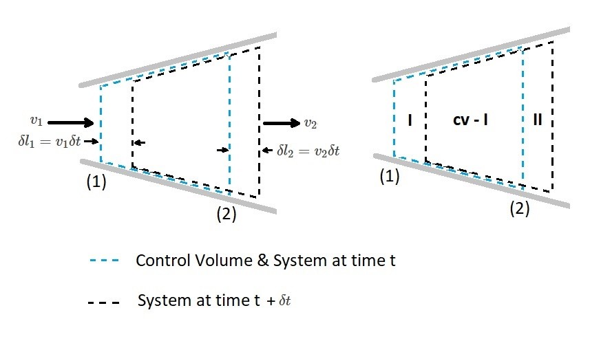
From the above image the outflow for the system is represented by volume II, while the inflow of the system is represented by volume I. In addition the control volume is represented by CV. Hence, at time $t$, SYS = CV. On the other hand at time $t+δt$ the system is now (CV-1)+II. As a result SYS = CV-1+II.
$B_{sys}(t) = B_{CV}(t)$
Where B is an extensive parameter of the system. To further elaborate using $t+δt$:
$B_{sys}(t+δt)=B_{CV}(t+δt)B_1(t+δt)+B_{II}(t+δt)$
In order to change the amount of B in the system we will have to divide δt by the time interval. Also remember that we are saying $B_{sys}(t) = B_{CV}(t)$ As a result we will obtain the following equation.
(Eq 5) $\frac{δB_{sys}}{δt}= \frac{B_{CV}(t+δt)-B_{CV}(t)}{δt}-\frac{B_1(t+δt)}{δt}+\frac{B_{II}(t+δt}{δt}$
Next, if we were to use the limit $δt→0$, the left hand side of equation 5 will be equal to the time rate of change of B for the system. This is denoted as $DB_{sys}/Dt$. In turn this makes use of the material derivative notation, $D()/Dt$, used to emphasize the Lagrangian character of the time rate of change.
Let’s take a look at the first term on the right side of equation 5. The first term represents the time rate of change within the control volume. If we take the limit $δt→0$, the first term of equation 5 will become the following.
(Eq 6) $\lim_{δt\to 0} \frac{B_{CV}(t+δt-B_{CV}(t)}{δt}=\frac{∂B_{CV}}{∂t}=\frac{∂(\int{_{CV}}ρbdV)}{∂t}$
Now let’s take a look at 3rd term of equation 5. This term represents the rate that B flows from the control volume across the control surface. This is represent by the amount per unit volume, $ρb$, times the volume.
$B_{II}(t+δt)=(ρ_2b_2)(δv_{II}) = ρ_2A_2v_2b_2δt$
Next the limit $δt→0$ can be applied to the 3rd term of equation 5 resulting in the following equation.
(Eq 7) $\dot{B}_{out}=\lim_{δt\to 0}\frac{B_{II}(t+δt}{δt}=ρ_2A_2v_2b_2$
In addition the same statements can be applied to 1st part of equation 5. However, instead of representing the rate B flows from the control volume, it will represent the rate B flows into the control volume.
(Eq 8) $\dot{B}_{in}=\lim_{δt\to 0}\frac{B_{I}(t+δt}{δt}=ρ_1A_1v_1b_1$
Finally, after combining equation 5 – 8 we will obtain a version of the Reynolds Transport Theorem.
(Eq 9) $\frac{DB_{sys}}{Dt}=\frac{∂B_{CV}}{∂t}+\dot{B}_{out}-\dot{B}_{in}$
Reynolds Transport Theorem General Conditions
Equation 9 is a simplified version of the Reynolds transport theorem representing one dimensional mass flow rate through a control volume. However, the flow can become more complex, such as if it were unsteady or a three-dimensional flow. In those cases its is better to know what the general form of the Reynolds transport theorem is.
What ever the case is we will still need to consider the fluid within a control volume at time t. Than after a short time period has passed will need to consider the fluid that has exited as well as entered the control volume. Again we will consider the extensive fluid property B. Where again we will need to consider how the rate of change of B associated with the system is also related to how B changes within the control volume at any given time.
It also important to consider that a control volume can contain more (or less) than one inlet and outlet. For example a piping can system can have multiple inlets and outlets. What is important is that we correctly interpret the terms $\dot{B}_{in}$ and $\dot{B}_{out}$. Where $\dot{B}_{in}$ represents the net flow in to the control volume and $\dot{B}_{out}$ represents the net flow out.
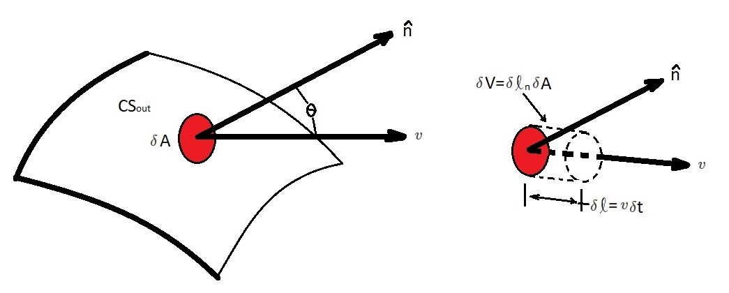
Let’s take a look at the image above. The image above represent the outflow portion of the control surface, $CS{out}$. $δA$ is an infinitesimal area element on the control surface. The volume of fluid passing through $δA$ is represented by $δV=δl_nδA$. In addition $δl_n=δl cosθ$ is the height that is normal to $δA$, where θ is the angle between the velocity vector and outward pointing normal to the surface $\hat{n}$. As a result $δl=vδt$, which is the amount of B moving through $δA$ within a certain time interval $δt$.
$δB = bρδV = bρ(vcosθδt)δA$
Next applying the limit $δt→0$ while the fluid property B moves through $δA$ of the control volume will result in the following.
$δ\dot{B}_{out} = \lim_{δt\to 0}\frac{ρbδV}{δt}=\lim_{δt\to 0}\frac{(ρbv~cos~θ~δt)δA}{δt} = ρbv~cos~θ~δA$
After that we will need to integrate the entire outflow portion moving through the control surface $CS_{out}$.
$\dot{B}_{out} = \int{_{CS_{out}}}~d\dot{B}_{out}=\int{_{CS_{out}}}~ρbv~cos~θ~dA$
The velocity component $v~cos~θ$ is normal to the area element $δA$. As a result $v~cos~θ~= v·\hat{n}$. Hence the above equation can be modified to the following.
(Eq 10) $\dot{B}_{out} =\int{_{CS_{out}}}~ρbv·\hat{n}dA$
Similar steps would be taken to determine inflow portion of the control volume. The following equation would result.
(Eq 11) $\dot{B}_{in} =-\int{_{CS_{in}}}~ρbv·\hat{n}dA$
Next, equation 10 and 11 can be combined to result in the following equation.
(Eq 12) $\dot{B}_{out} – \dot{B}_{in} = \int{_{CS}}~ρbv·\hat{n}dA$
This will allow an integration over the entire control surface. Next equation 12 will need to be combined with equation 9 in order to consider the fluid inside the control volume.
$\frac{DB_{sys}}{Dt}=\frac{∂B_{CV}}{∂t}+\int{_{CS}}~ρbv·\hat{n}dA$
or
(Eq 13) $\frac{DB_{sys}}{Dt}= \frac{∂}{∂t}\int{_{CV}}~ρbV +\int{_{CS}}~ρbv·\hat{n}dA$
Equation 13 represents the general form of Reynolds transport theorem for control volume that is fixed and non deforming.
The Purpose of Reynolds Transport Theorem
First, the Reynolds transport theorem is widely used in fluid mechanics. As a result it is important that you have an understanding of what its purpose is. The main purpose of the Reynolds transport theorem is to provide a way to link control volume ideas and system idea.
The left side of equation 13 purpose is to provide an arbitrary extensive parameter that is the time rate of change of a system. For example this could be mass, momentum, energy, etc. It all depends what you want the parameter B to represent.
Remember that a system is moving. While on the other hand a control volume is stationary. Hence the amount of B within the control volume isn’t always equal to the system. The first term in equation 13 represents fluid flowing through the control volume. As a result, the rate of change of B inside the control volume can be determined.
Finally, the last term in equation 13 represents the net flowrate of B over entire control surface. Hence it is determine how much fluid is entering and leaving the control volume.
Steady State
If the flow going through the control volume is in a steady state, than equation 13 can be reduced to the following equation.
(Eq 14) $\frac{DB_{sys}}{Dt}=\int{_{CS}}~ρbv·\hat{n}dA$
What this means is the following. First, there is a certain quantity of B in relation to the system. This in turn would have be related to the control volume. B is related to the control volume where there is a net difference in rate the B flows into and out of the control volume. In other words the flow rate in must be the same as the flow rate out. In addition when the flow is steady the property B within the control volume does not change with time. However, the amount of the property B associated with the system may or may not change with time. In steady, for a system, it will depend what particular property is being considered.
Unsteady State
Now if the flow were in an unsteady condition than $∂(~)/∂t≠0$. As a result all of terms within equation 13 will need to be used unless its a special case. Hence for both the system and the control volume the parameter B may change with time.
As mentioned above there is a special situation where equation 13 can be reduced even if the flow is unsteady. This can occur if the rate of the inflow of parameter B is balanced by the rate of out flow. In other words $\int{_{CS}}~ρbv·\hat{n}dA = 0$. When this is the case equation 13 can be reduced to the following.
(Eq 15) $\frac{DB_{SYS}}{Dt}=\frac{∂}{∂t}\int{_{CV}}~ρbdV$
As a result the rate of change of B of the system is the same as the rate of change of B within the control volume.