Generally when you are solving a fluid mechanics problem you can use a fixed control volume. However, there can be cases when you will need to have a moving control volume. For example if you wanted to analyze a jet engine, or a rocket, you will need to use a moving control volume. In certain cases the control volume itself may even deform. Such as if you were analyzing a deflating balloon that was moving around a room after you let go of it. Depending on what you are looking at, moving control volumes can become complex.
Moving Control Volume
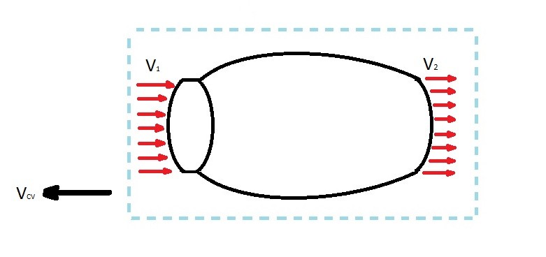
Let’s take a look at the image above. In the image there is a sketch of a jet engine. At its inlet, air is moving into the engine at velocity $v_1$. While at its outlet, air is moving out of the engine at a velocity $v_2$. As the air moves through the engine a force will be created. In turn, this force will push the engine and what ever is attached to the engine in the opposite direction of air going through the engine. In order to analyze the engine, the control volume will have to move with the engine at the same velocity. The velocity of the control volume is represented by the variable $v_{CV}$.
When you are solving this type of problem you will need to realize that there is a relative velocity as well as an absolute velocity. As with a stationary control volume, there is a fluid that is moving through the control volume. However, in this case, the control volume is moving. Hence, the relative velocity of the fluid is the fluid moving through the control volume. The reason why is because if an observer were sitting on the engine they would only be able to observe the fluid moving through the engine. On the other hand if you had a fixed observer, they will be able to see the absolute velocity of the fluid moving through the engine. To determine the absolute velocity of the fluid you would use the following equation.
(Eq 1) $v = W + v_{CV}$
$W$ = relative velocity
$v_{CV}$ = velocity of the control volume
Be aware that the velocity of the fluid moving through the control volume is generally different than the velocity of the control volume. For example, lets say for simplicity both $v_1$ and $v_2$ for the jet engine both equal $100\frac{ft}{s}$, and the control volume is moving at a velocity of $-20\frac{ft}{s}$. If this is the case than the absolute velocity of the fluid is $100 – 20 = 80\frac{ft}{s}$.
Moving Control Volumes and Reynolds Transport Theorem
In a previous article I discussed Reynolds transport theorem for a non-deforming, fixed control volume. It can however be modified so that it can be used to relate a system to a non-deforming, moving control volume. This will result in the following equation. Remember that “B” represents some extensive property of the system and “b” is an intensive property.
(Eq 2) $\frac{DB_{sys}}{Dt} = \frac{∂}{∂t}~\int{_{CV}}~ρbdV + \int{_{CS}}~ρbW·\hat{n}dA$
$ρ$ = fluid density
$V$ = volume
$A$ = Area