The energy equation is an application of the first law of thermodynamics. It states the following. The time rate of increase of the total stored energy within the system will equal the net time rate of energy added due to heat transfer into the system, plus, the time rate of energy added to the system due to work. Therefore, the following equation will represent the first law of thermodynamics in regards to the energy equation.
(Eq 1) $\frac{D}{Dt}~\int{_{sys}}~eρdV=(\sum{\dot{Q}_{in}}-\sum{\dot{Q}_{out}})+(\sum{\dot{W}_{in}}-\sum{\dot{W}_{out}})$
The First Law of Thermodynamics & the Energy Equation
To derive the energy equation you will need to have an understanding of what equation 1 means, and how to apply it to a control volume.
Energy Term
First, let’s talk about the variable “$e$” in the above equation. The variable “$e$” represents the total stored energy per unit mass that is in the system for each particle. As a result $”e”$ is related to the internal energy per unit mass, kinetic energy per unit mass, and the potential energy per unit mass. This will result in the following equation.
(Eq 2) $e = \check{u} + \frac{v^2}{2}+gz$
$\check{u}$ = internal energy per unit mass
$v$ = velocity
$g$ = gravitational constant
$z$ = fluid height
If you haven’t noticed equation 2 is starting to take the form of the Bernoulli Equation.
Heat Transfer and Work
The next term of equation 1, $(\sum{\dot{Q}_{in}}-\sum{\dot{Q}_{out}})$, represents the rate of the heat transfer into the system. This term can also be denoted as $\dot{Q}_{net,~in}$. On the other hand, the following term, $(\sum{\dot{W}_{in}}-\sum{\dot{W}_{out}})$, represents the net rate of work that is being transferred into the system. Likewise, this term can be denoted as $\dot{W}_{net,~in}$. Both heat transfer and work transfer will be “+” when they enter the system, and “-” as they exit. However, to further develop equation 1, we will need to relate the heat transfer and work of the system to a control volume. In turn this will result in the following equation.
(Eq 3) $(\dot{Q}_{net~in}+\dot{W}_{net~in})_{sys} = (\dot{Q}_{net~in}+\dot{W}_{net~in})_{CV}$
Using Reynolds Transport Theorem
In order to relate a system to a coincident control volume Reynolds transport theorem is used, where the parameter “$b$” of the Reynolds transport theorem will equal “$e$”.
(Eq 4) $\frac{D}{Dt}~\int{_{sys}}~eρdV = \frac{∂}{∂t}~\int{_{CV}}~eρdV + \int{_{CS}}~eρv·\hat{n}dA$
$ρ$ = density
As a result, the Reynolds transport theorem will allow us to state the following. The time rate of increase of the total stored energy within the system will equal the time rate of increase of the total energy within the control volume, plus, the net rate of flow of the total energy moving out of the control through the control surface.
Finally, after combining equations 1, 3, and 4, the formula for the first law of thermodynamics in regards to a control volume will be defined as,
(Eq 5) $ \frac{∂}{∂t}~\int{_{CV}}~eρdV + \int{_{CS}}~eρv·\hat{n}dA = (\dot{Q}_{net~in}+\dot{W}_{net~in})_{CV}$
In equation 5 $”e”$ is the total energy per unit mass for fluid particles that leaving, entering, and within the control volume. On the other hand “$\dot{Q}$” represents every way that energy can exchanged between the surroundings and the control volume due to a temperature difference. Hence all types of heat transfer, conduction, convection, and radiation will apply. Finally, since heat transfer into the control volume is positive and heat transfer out of the control volume is negative, an adiabatic process will result in a net heat transfer rate of zero through the control volume. In addition, $”\dot{W}”$ represents power. Power is positive when work done on the contents of control volume by the surroundings.
Work Caused by a Shaft
There are many different ways that work can be transferred across the control surface. One way is a moving shaft. Some devices that use a moving shaft are fans, propellers, and turbines. What ever the case, work enters the control volume where the control surface slices through the shaft.
In order to calculate work, you need to take the dot product of a force and the total displacement caused by the force. As a result, power is force related to displacement per unit time. To further this, since a shaft is a rotating object, the work caused by a shaft will be related to the shafts torque “$T$”. While the power will be a product of the torque on the shaft times the angular velocity “$ω$”. Hence, $\dot{W}_{shaft} = T_{shaft}ω$. Finally, if a shaft, or multiple shafts, were cutting through the control surface, there will be a net work on the control surface as seen in the following equation.
(Eq 6) $\dot{W}_{shaft~net~in} = \sum{\dot{W}_{shaft~in}} – \sum{\dot{W}_{shaft~out}}$
Work caused by Fluid Flowing Through a Simple Pipe
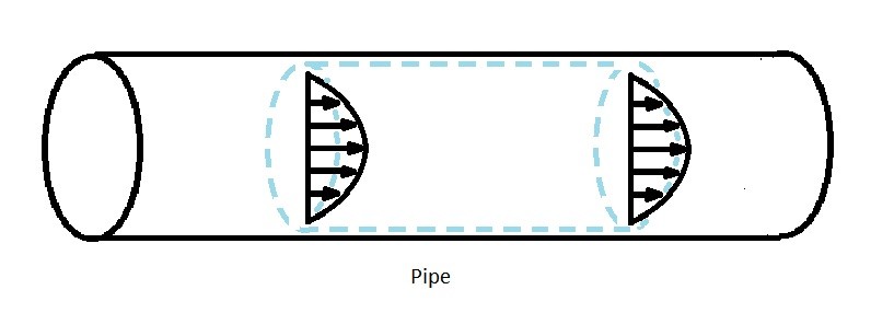
Work can can also be transferred through a control surface through normal force that is acting over a distance. For example fluid within a simple pipe will create a normal stress “$σ$” on the pipe due to the fluid pressure $”p”$.
(Eq 7) $σ=-p$
Power transfer, “$\dot{W}$ is also associated with a force “$F$” that is acting on a moving object at a certain velocity “$v$”. This can be calculated using a dot product. As stated above, work transferred through a control surface can be caused by a normal force. Hence, $ð\dot{W}_{normal~stress} = δF_{normal~stress} · v$ Taking this and equation 7 into consideration the power caused by a normal stress can be calculated using the following equation.
(Eq 8) $δ\dot{W}_{normal~stress} = σ\hat{n}δA·v = -p\hat{n}δA·v = -pv·\hat{n}δA$
or
$\dot{W}_{normal~stress} = \int{_{CS}}~σv·\hat{n}dA = \int{_{CS}}~-pv·\hat{n}dA$
Going back to a simple pipe, let’s take a look at $\dot{W}_{normal~stress}$ where fluid contacts the surface of the pipe. At these points $\dot{W}_{normal~stress}$ will equal zero. As a result it will only have a non-zero value where the fluid enters and leaves the control volume.
In addition to normal stress there can also be a tangential stress that is acting on the control surface. As a result the work transfer equation for tangential stress will be similar to the equation that was used for a normal stress.
(Eq 9) $δ\dot{W}_{tangential~stress} = δF_{tangential~stress}·v$
Again looking at the simple pipe, the velocity at the wall of the pipe will be zero. This happens to be where the control volume is placed. As a result $\dot{W}_{tangential~stress}$ will also equal zero.
Energy Equation
Finally, using the information about power that was developed above, we can generate an equation that represents the first law of thermodynamics for the contents of a control volume. This equation is derived by combining equations 5, 6, and 8.
(Eq 10) $\frac{∂}{∂t}~\int{_{CV}}~eρdV + \int{_{CS}}~eρv·\hat{n}dA = \dot{Q}_{net~in} + \dot{W}_{shaft~net~in}-\int{_{CS}}~pv·\hat{n}dA$
Finally, the energy equation is derived by combining equation 10 with equation 2.
(Eq 11) $\frac{∂}{∂t}~\int{_{CV}}~eρdV + \int{_{CS}}~\left(\check{u} + \frac{p}{ρ}+\frac{v^2}{2}+gz\right)ρv·\hat{n}dA = \dot{Q}_{net~in} + \dot{W}_{shaft~net~in}$
Applying the Energy Equation
In equation 11 the term $\frac{∂}{∂t}~\int{_{CV}}~eρdV$ represents the total stored energy change in respect to time. If the flow is steady, this term will become zero, allowing you to remove it from the equation. This statement also applies if the mean of the flow is steady, or in other words if an unsteady flow is cyclical.
Next, the integrand $ \int{_{CS}}~\left(\check{u} + \frac{p}{ρ}+\frac{v^2}{2}+gz\right)ρv·\hat{n}dA$ is nonzero only where the fluid crosses the control volume. In other words, $(v·\hat{n} ≠ 0)$. Any where else on the control surface $(v·\hat{n} = 0)$, making this term of the equation equal zero. In addition, if you can assume that the term $\hat{u}$, $p/ρ$, $v^2/2$, and $gz$ are uniformly distributed, than this term can be modified to the following equation.
(Eq 12) $\int{_{CS}}~\left(\check{u} + \frac{p}{ρ}+\frac{v^2}{2}+gz\right)ρv·\hat{n}dA =$$ \sum{_{flow~out}}~\left(\check{u} + \frac{p}{ρ}+\frac{v^2}{2}+gz\right)\dot{m}$$ – \sum{_{flow~in}}~\left(\check{u} + \frac{p}{ρ}+\frac{v^2}{2}+gz\right)\dot{m}$
To further this statement, if one stream of fluid was entering and exiting the control volume, than equation 12 can be reduced the following equation.
(Eq 13) $\int{_{CS}}~\left(\check{u} + \frac{p}{ρ}+\frac{v^2}{2}+gz\right)ρv·\hat{n}dA =$$ \left(\check{u} + \frac{p}{ρ}+\frac{v^2}{2}+gz\right)_{out}\dot{m}_{out}$$ – \left(\check{u} + \frac{p}{ρ}+\frac{v^2}{2}+gz\right)_{in}\dot{m}_{in}$
These equations can only be applied to uniform flow. Generally, in reality, uniform flow can only occur through an infinitesimally small diameter. As a result, to use these equations, you will need to idealize the actual conditions so that you disregard nonuniformities. This in turn is known as one dimensional flow, and is used to simplify the problem.
Work on a Shaft
Finally, if you are analyzing work caused by a shaft, the flow will be unsteady, or at least unsteady locally. Hence, flow within a machine that has shaft work will be unsteady. On the other hand, if you were to analyze the flow down or upstream from the shaft, flow may be steady, or can be assumed to be steady. If you were to analyze the flow as if it were one-dimensional, cyclical, with one stream entering and leaving the control volume, for an average time basis, than the energy equation would become the following.
(Eq 14) $\dot{m} \left[\check{u}_{out} – \check{u}_{in} + \left(\frac{p}{ρ}\right)_{out} – \left(\frac{p}{ρ}\right)_{in} + \frac{v^2_{out}-v^2_{in}}{2}+g(z_{out}-z_{in})\right]$$=\dot{Q}_{net~in}+\dot{W}_{shaft~net~in}$
Next, the fluid property enthalpy, $\check{h}$, is calculated using the following equation.
(Eq 15) $\check{h} = \check{u} + \frac{p}{ρ}$
In turn, equation 15 can be inserted into equation 14.
(Eq 16) $\dot{m} \left[\check{h}_{out} – \check{h}_{in} + \frac{v^2_{out}-v^2_{in}}{2}+g(z_{out}-z_{in})\right]$$=\dot{Q}_{net~in}+\dot{W}_{shaft~net~in}$
Finally, if the flow is steady throughout the control volume, you are analyzing the problem as a one-dimensional flow, and one flow stream is entering and exiting the control volume, than shaft work will go to zero. As a result equation 16 will reduce the following.
(Eq 17) $\dot{m} \left[\check{h}_{out} – \check{h}_{in} + \frac{v^2_{out}-v^2_{in}}{2}+g(z_{out}-z_{in})\right]$$=\dot{Q}_{net~in}$