When you apply a moment of a force around an axis you will generate a torque. In turn, for a fluid, the linear momentum of a fluid particle can be used to determine a torque. In the process of doing this we will develop a moment of a momentum equation. As a result, this will allow us to relate torques to the angular momentum of a flow in regards to the contents of a control volume. Hence, as with linear momentum, Newton second law, seen in equation 1, is used to determine the moment of a momentum equation.
(Eq 1) $\frac{D}{Dt}(vρδV) = δF_{particle}$
$v$ = particle velocity
$ρ$ = density
$V$ = volume
$F$ = resultant external force
Deriving the Moment of a Momentum Equation
To derive the moment of a momentum equation you will first need to place a moment on each side of equation 1.
(Eq 2) $r×\frac{D}{Dt}(vρδV) = r×δF_{particle}$
$r$ = position vector
In the above equation “$r$” is the position vector in regards to the origin of the inertial coordinate system. In addition, we can also state the following.
(Eq 3) $\frac{D}{Dt}[(r×v)ρδV] = \frac{Dr}{Dt}×vρδV+r×\frac{D(vρδV)}{Dt}$
(Eq 4) $\frac{Dr}{Dt} = v$
(Eq 5) $v×v = 0$
As a result, we can combine equations 2-5 to obtain the following equation.
(Eq 6) $\frac{D}{Dt}[(r×v)ρδV] = r×δF_{particle}$
In regards to a system, equation 6 will be valid for all fluid particles. However, when analyzing a system we will need to sum both sides of equation 6. Hence, the following equation will result.
(Eq 7) $\int{_{sys}}~\frac{D}{Dt}[(r×v)ρdV] = \sum{(r×F)_{sys}}$
where,
(Eq 8) $\sum{r×δF_{particle}}=\sum{(r×δF)_{sys}}$
In addition, we can note that,
(Eq 9) $\frac{D}{Dt}\int{_{sys}}~(r×v)ρdV=\int{_{sys}}~\frac{D}{Dt}[(r×v)ρdV]$
The is sequential order of differentiation and integration is showing that it can reversed without any consequences. As a result,
(Eq 10) $\frac{D}{Dt}\int{_{sys}}~(r×v)ρdV = \sum{(r×δF)_{sys}}$
What this is saying is the following. In regards to the moment of a momentum of a system, the time rate of change will equal the sum of all external torques that are acting on the system. However, this statement will have to be instantaneously coincident with a control volume. As a result the torques acting on the system as well as the control volume will be identical. Hence,
(Eq 11) $\sum{(r×δF)_{sys}}=\sum{(r×δF)_{CV}}$
Next, the Reynolds transport theorem can be used to relate the system and contents of control volume to determine the moment of a momentum equation for a fixed, non-deforming control volume.
(Eq 12) $\frac{D}{Dt}~\int{_{sys}}~(r×v)ρdV = \frac{∂}{∂t}~\int{_{CV}}~(r×v)ρdV + \int{_{CS}}~(r×v)ρv·\hat{n}dA$
Equation 12 is stating the following. First, on the left side of equation it is describing time rate of change for the moment of a momentum of a system. In turn, this will be equal the time rate of change of the moment of a momentum for the contents of the control volume, plus the net rate of flow through control surface of the moment of the momentum. Finally, equations 10-12 are combined. This will result in the moment of a momentum equation.
(Eq 13) $\frac{∂}{∂t}~\int{_{CV}}~(r×v)ρdV + \int{_{CS}}~(r×v)ρv·\hat{n}dA = \sum{(r×F)}_{CV}$
This equation will give you the ability to solve problems that involve machines that rotate. Some examples include, rotary lawn sprinklers, ceiling fans, and turbochargers. In other words, the moment of a moment equation will allow to solve problems related to devices that are called turbo-machines.
Application of the Moment of a Momentum Equation
When you are using the moment of a momentum equation there are few things that you can look at to help simplify the equation.
- Make the Flow One-Dimensional
First, one assumptions that can be made is that the flow is one-dimensional. By doing this we can say that there is a uniform distribution of average velocity at any section of the control volume.
-
Steady Flow
Second, if you are able to say the flow is steady you will be able to simplify the moment of a momentum equation.
$\frac{∂}{∂t}~\int{_{CV}}~(r×v)ρdV=0$
In addition, this simplification of the equation can also be used on time-average basis for cyclical unsteady flows.
-
One Dimensional Steady Flow through a Rotating Machine
The moment of a momentum equation is used quite often for objects rotating around an axis of rotation. An example of this would be a rotating sprinkler head, which can be seen in the image below.
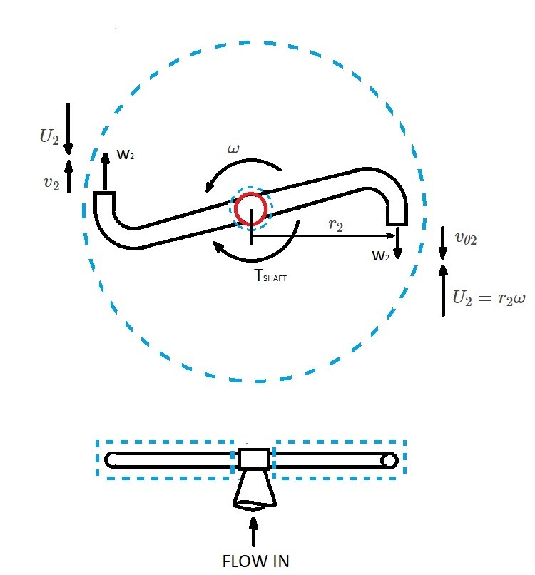
As the water exits the sprinkler head a momentum will result. Consequently, this momentum will exert a torque on the sprinkler. Therefore, the sprinkler head will start to rotate because of momentum of the exiting fluid. However, the resulting torque will limit how fast the sprinkler can rotate.
In order to analyze the sprinkler head a control volume will need to be used. In this case, a fixed, non-deforming control volume will be used. The control volume is illustrated by the blue dotted lines in the above image. Be aware that the control surface cuts through sprinkler head near the axis of rotation. The reason for this is to identify the torque cause by the momentum of the water. In order to analyze the sprinkler head we will need to use the axial component of the moment of a momentum equation seen in equation 13.
First, we will need to take a look at the integrand of the moment of a momentum flow term.
$\int{_{CS}}~(r×v)ρv·\hat{n}dA$
At the point where the fluid is crossing the control surface the flow term will be a nonzero value. However, at every other point this term will be zero because $v·\hat{n}dA=0$.
For the sprinkler head the water will enter through the stem. At this point the control surface of the control volume is located at the axis of rotation. As a result $r×v$ will go to zero at the axis of rotation. Therefore there will no axial moment of a momentum at the axis of rotation.
Next, the water will exit through two nozzle openings. In this case the $r×v$ will not equal zero. Instead it will equal $r_2v_{θ2}$ where v_{θ2} is the tangential component of the flow exiting the nozzles and $r_2$ is the radius of rotation from the axis of rotation to the nozzle’s center-line. Furthermore, you need to be aware that the fluid velocity leaving the nozzles will be a relative velocity “W”. Due to this fact, you will need to relate the relative velocity of the fluid to the absolute velocity “$v$” of the fluid in respect to the fixed control surface.
(Eq 14) $v = W+U$
$v$ = absolute velocity
$W$ = relative velocity
$U$ = velocity of the moving nozzle measured relative to the fixed control surface
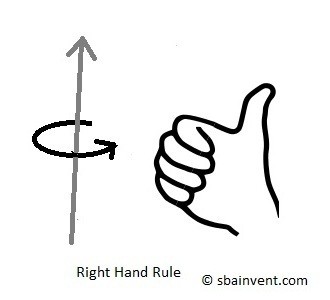
Next, we need to determine what will be negative and what will positive terms in relation to $\int{_{CS}}~(r×v)ρv·\hat{n}dA$. When the flow is exiting the control volume, $v·\hat{n}$ will be positive. On the other hand, when the flow enters the control volume, $v·\hat{n}$ will be negative. In addition to the dot product, we will also need to consider the cross product $r×v$. Because this is considering whether the rotations about the fixed axis is positive or negative we will need to refer to the right hand rule. The image below shows a positive rotation according to the right hand rule.
Taking all of this in to consideration the flow term of the moment of a momentum equation, for a rotating sprinkler head, can be expressed as the following.
(Eq 15) $[\int{_{CS}}~(r×v)ρv·\hat{n}dA]_{axial} = (-r_2v_{θ2})(+\dot{m})$
$\dot{m}$ = total mass flowrate through both nozzles
In addition to the flow term of the moment of a momentum equation, we will also need to discuss the torque term $\sum{(r×F)}_{CV}$. To start we will need to confine ourselves to the torques that are acting on axis of rotation only. These torques will be associated with normal forces that are exerting themselves onto the contents within the control volume. We will not need to consider any net axial torques that are the result of fluid tangential forces because they are normally negligibly small. As a result the torque term for the mass moment of a momentum equation will become the following.
(Eq 16) $\sum{[(r×F)_{CV}]}_{axial} = T_{shaft}$
As with the direction of the flow, to determine if the torque is positive or negative the right hand rule would used. However, the torque’s direction is always in the opposite direction of the rotation of the sprinkler head. Finally, equations 15 and 16 can be combined to determine the axial component of the moment of a momentum equation.
(Eq 17) $-r_2v_{θ2}\dot{m}=T_{shaft}$
Now that we know what the torque is at axis of rotation, we can determine the power “$\dot{W}$” that fluid is generating for a specific angular velocity.
(Eq 18) $\dot{W}_{shaft} = T_{shaft}ω = -r_2v_{θ2}ω = -U_2v_{θ2}\hat{m}$
$ω$ = angular velocity
Finally, work per unit mass “$w_{shaft}$” can be determine using the following equation.
(Eq 19) $w_{shaft} = -U_2v_{θ2}$
The equations that were derived for the sprinkler head example can be used for most simplified turbo-machine flows.
-
General, One Dimensional Steady Flow through a Rotating Machine
The equations that were derived for the sprinkle head example can take on more general form. First, to determine the torque around the axis of rotation, the general equation would be the following.
(Eq 20) $T_{shaft} = (-\dot{m}_{in})(±r_{in}v_{θin})+\dot{m}_{out}(±r_{out}v_{θout})$
In addition, the power being generated around the axis of rotation can be described by the following equation.
(Eq 21) $\dot{W}_{shaft} = (-\dot{m}_{in})(±r_{in}ωv_{θin})+\dot{m}_{out}(±r_{out}ωv_{θout})$
Finally, to determine the work per unit mass around the axis of rotation the following equation would be used.
(Eq 22) $w_{shaft} = -(±U_{in}v_{θin})+(±U_{out}v_{θout})$